Industry Leaders US: Top 3 Revenue Companies in Every Growing


Contents
- The Strategy
- Methodology
- Results
- What the Pattern Shows
- Why the Alpha Disappeared
- Run It Yourself
- Limitations
Revenue leaders have structural advantages. They set prices, not take them. They have scale that compounds. Their access to capital is cheaper than everyone else's in their industry. The question is whether those advantages show up in stock returns.
We built a backtest to find out: take the 3 largest companies by revenue in every US industry that's actively growing, hold them equally weighted, rebalance each July. Run it from 2001 to 2025. Here's what 24 years of data shows.
The Strategy
Signal: Two conditions at each annual rebalance in July: 1. Industry average YoY revenue growth >= 5% (excludes declining or stagnant industries) 2. Company is in the top 3 by current FY revenue within that qualifying industry
Portfolio: Equal weight across all qualifying stocks. Maximum 300 positions.
Universe: NYSE, NASDAQ, and AMEX. Not S&P 500 constrained. Full exchange coverage with a $1B market cap floor.
Rebalance: Annual, each July. Uses financials filed at least 45 days prior to avoid look-ahead bias.
The result at any given July is typically 150-230 stocks representing the revenue-dominant companies across every growing corner of the US economy.
Methodology
- Universe: NYSE, NASDAQ, AMEX (all actively traded)
- Market cap filter: $1B+ USD at each rebalance date
- Rebalancing: Annual (July), using FY financial data with 45-day filing lag
- Portfolio size: Up to 300 stocks, equal weight. Cash when fewer than 10 qualify.
- Industry growth threshold: Average industry YoY revenue growth >= 5%
- Min industry size: 3 companies required to identify a "leader"
- Leaders per industry: Top 3 by current FY revenue
- Transaction costs: Size-tiered model based on market cap at time of trade
- Data period: July 2001 through July 2025 (24 annual periods)
- Benchmark: SPY (S&P 500 ETF)
- Data source: Ceta Research FMP financial data warehouse
Full methodology at backtests/METHODOLOGY.md.
Results
| Metric | Industry Leaders US | SPY |
|---|---|---|
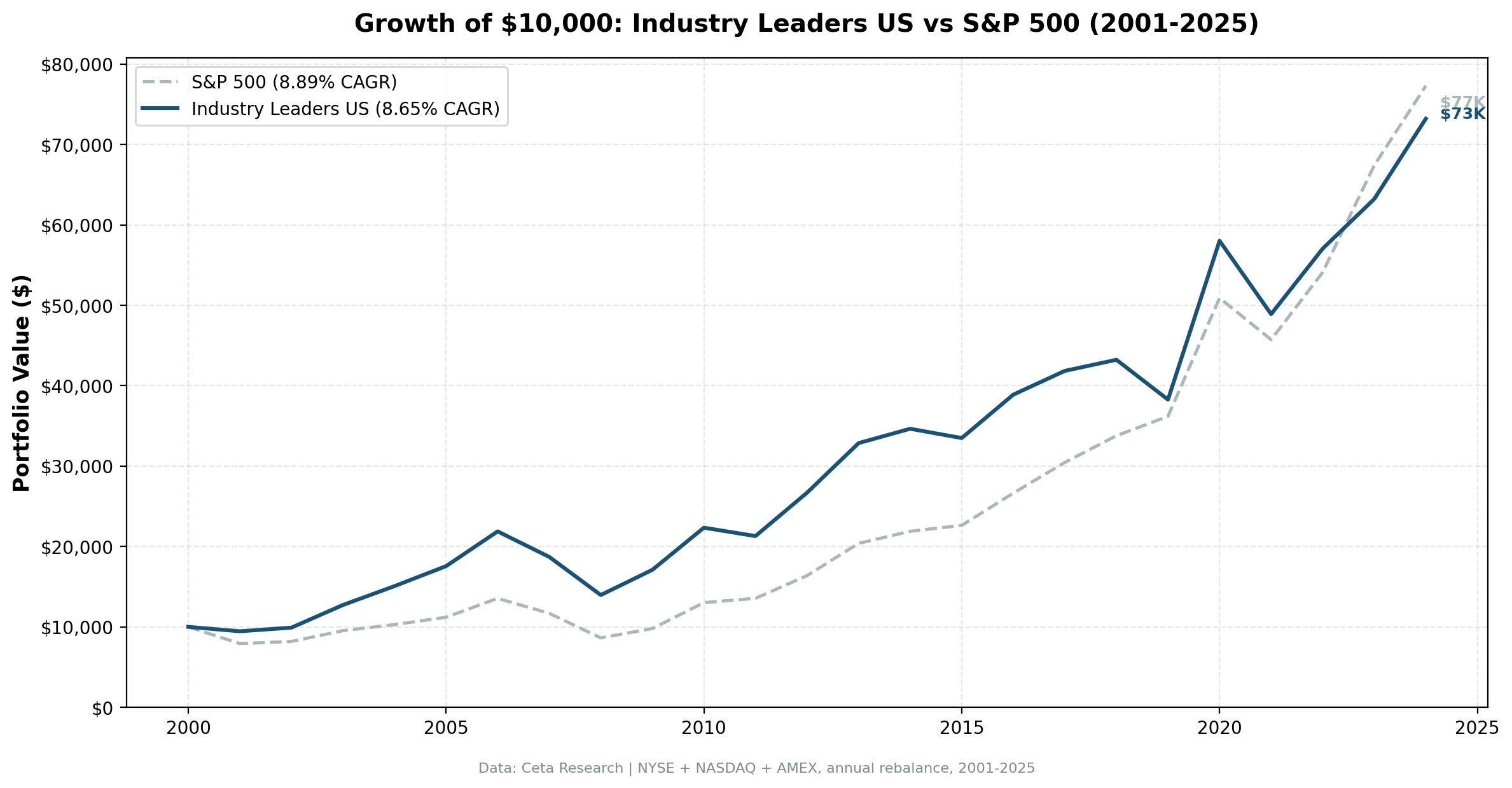
| CAGR | 8.65% | 8.89% |
| Total return (24yr) | 631.8% | 672.9% |
| $10,000 grows to | $73,183 | $77,292 |
| Max drawdown | -36.19% | — |
| Invested periods | 24 of 24 | — |
| Avg holdings | ~229 stocks | — |
The strategy returned 8.65% annually vs 8.89% for SPY, a -0.25% annual gap over 24 years. In dollar terms: $10,000 in 2001 grew to $73,183 vs $77,292 for SPY.
That's the headline. But the story is more interesting than the number.
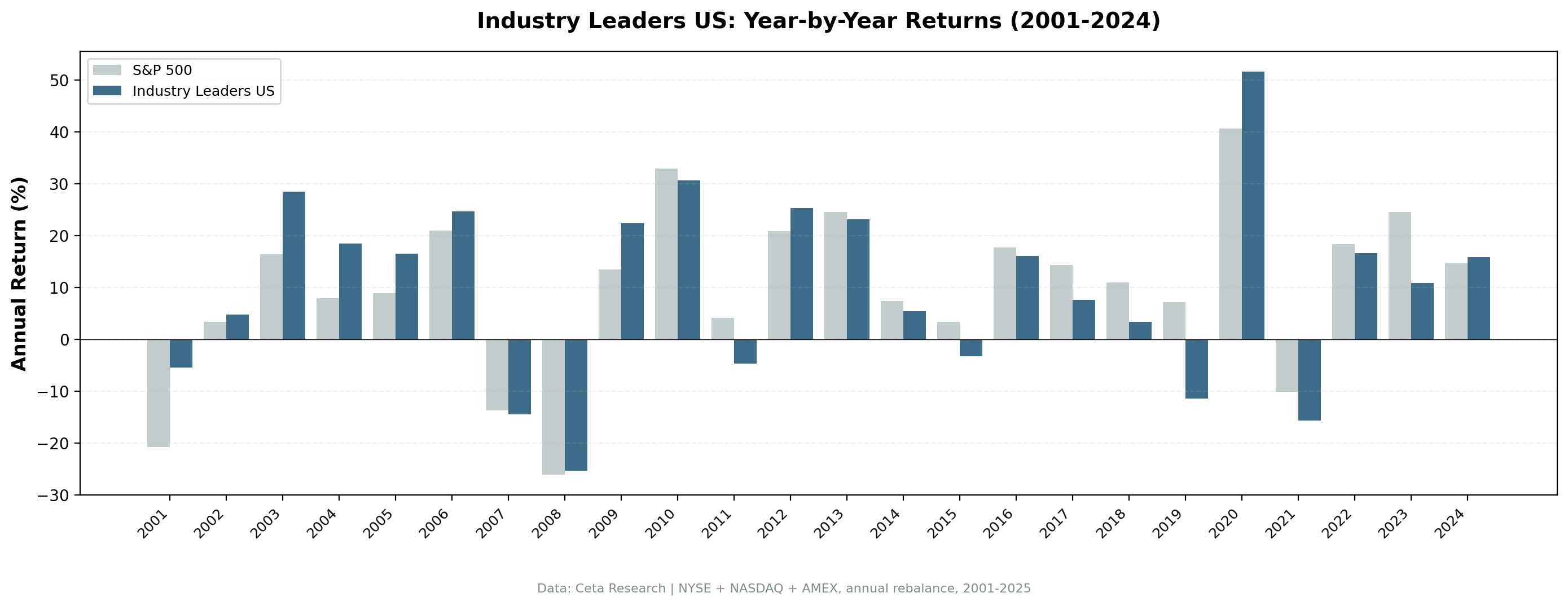
Annual returns:
| Year | Portfolio | SPY | Excess |
|---|---|---|---|
| 2001 | -5.49% | -20.77% | +15.28% |
| 2002 | +4.78% | +3.29% | +1.49% |
| 2003 | +28.47% | +16.44% | +12.03% |
| 2004 | +18.44% | +7.94% | +10.50% |
| 2005 | +16.51% | +8.86% | +7.65% |
| 2006 | +24.61% | +20.95% | +3.66% |
| 2007 | -14.50% | -13.71% | -0.79% |
| 2008 | -25.36% | -26.14% | +0.78% |
| 2009 | +22.42% | +13.42% | +9.00% |
| 2010 | +30.69% | +32.94% | -2.25% |
| 2011 | -4.66% | +4.10% | -8.76% |
| 2012 | +25.33% | +20.85% | +4.48% |
| 2013 | +23.11% | +24.50% | -1.39% |
| 2014 | +5.43% | +7.38% | -1.95% |
| 2015 | -3.33% | +3.36% | -6.69% |
| 2016 | +16.12% | +17.73% | -1.61% |
| 2017 | +7.60% | +14.34% | -6.74% |
| 2018 | +3.30% | +10.91% | -7.61% |
| 2019 | -11.47% | +7.12% | -18.59% |
| 2020 | +51.63% | +40.68% | +10.95% |
| 2021 | -15.72% | -10.17% | -5.55% |
| 2022 | +16.66% | +18.31% | -1.65% |
| 2023 | +10.82% | +24.60% | -13.78% |
| 2024 | +15.80% | +14.67% | +1.13% |
Years are July-to-July periods (2001 = July 2001 to July 2002, etc.)
What the Pattern Shows
The first six years were strong. 2001 through 2006, the strategy beat SPY every single year. During the dot-com unwinding and subsequent recovery, holding companies with actual revenue made sense. Revenue leaders in manufacturing, financials, consumer goods, and energy all compounded well when growth stocks were getting repriced.
The middle years went sideways. 2011 through 2019 had more misses than hits. The strategy lagged in years when concentrated mega-cap returns drove SPY performance. If SPY's gains in a given year came from 10 stocks with massive market caps, a 229-stock equal-weighted revenue portfolio wouldn't capture those gains.
2019 was the worst year. -11.47% portfolio vs +7.12% SPY, a -18.59% gap. The July 2019 to July 2020 window included the COVID crash (Feb-Mar 2020). Revenue leaders in airlines, hospitality, retail, and energy got slammed. By July 2020, SPY had already recovered (healthcare and tech were heavily weighted), while the revenue-leader portfolio still carried beaten-down cyclical positions.
2020 was the strongest year. +51.63% vs +40.68%. The July 2020 to July 2021 period was a full recovery bounce. Revenue leaders across all industries snapped back after the COVID dislocation, and the equal-weighted construction meant every recovering industry contributed equally.
Why the Alpha Disappeared
The honest answer: when you hold the top 3 by revenue across every growing industry, you're running something close to an equal-weighted large-cap revenue index.
The US market has 100+ distinct industries. At each rebalance, the strategy holds about 229 stocks. Diversification at that level means individual winners barely move the needle, and the overall return reflects broad economic growth, not a concentrated bet on revenue leadership.
Academic research (Moskowitz & Grinblatt 1999) found industry momentum effects, and Hou (2007) documented information diffusion from revenue leaders to laggards. Those effects are real. But they're captured at the individual stock level, not the portfolio level when you're holding 229 names across the whole economy.
Two scenarios where the strategy should outperform: 1. Concentrated industries where 3 companies genuinely control a sector (the revenue moat is real) 2. Markets with high economic growth where revenue leaders compound disproportionately
The US market has thousands of companies across hundreds of industries. Competition is intense. Revenue leaders often face strong challengers. The moat is thinner than in concentrated markets.
Part of a Series: Global | India
Run It Yourself
Current screen (live data):
WITH latest_rev AS (
    SELECT i.symbol, p.industry, p.exchange, p.companyName,
        i.revenue, i.date AS filing_date,
        ROW_NUMBER() OVER (PARTITION BY i.symbol ORDER BY i.dateEpoch DESC) AS rn
    FROM income_statement i
    JOIN profile p ON i.symbol = p.symbol
    WHERE i.period = 'FY' AND i.revenue > 0
      AND p.industry IS NOT NULL AND p.industry != ''
      AND p.exchange IN ('NYSE', 'NASDAQ', 'AMEX')
),
prior_rev AS (
    SELECT i.symbol, i.revenue AS prior_revenue,
        ROW_NUMBER() OVER (PARTITION BY i.symbol ORDER BY i.dateEpoch DESC) AS rn
    FROM income_statement i WHERE i.period = 'FY' AND i.revenue > 0
),
company_growth AS (
    SELECT c.symbol, c.companyName, c.exchange, c.industry,
        c.revenue, p.prior_revenue, c.filing_date,
        (c.revenue - p.prior_revenue) / p.prior_revenue AS rev_growth
    FROM latest_rev c JOIN prior_rev p ON c.symbol = p.symbol
    WHERE c.rn = 1 AND p.rn = 2 AND p.prior_revenue > 0
),
company_filtered AS (
    SELECT cg.*, mc.marketCap FROM company_growth cg
    JOIN key_metrics_ttm mc ON cg.symbol = mc.symbol
    WHERE mc.marketCap >= 1000000000
),
industry_agg AS (
    SELECT industry, COUNT(*) AS n_companies,
        ROUND(AVG(rev_growth) * 100, 2) AS avg_growth_pct
    FROM company_filtered GROUP BY industry
    HAVING COUNT(*) >= 3 AND AVG(rev_growth) >= 0.05
),
leaders AS (
    SELECT cf.symbol, cf.companyName, cf.exchange, cf.industry,
        ROUND(cf.revenue / 1e9, 2) AS revenue_b,
        ROUND(cf.rev_growth * 100, 2) AS rev_growth_pct,
        ia.avg_growth_pct AS industry_growth_pct,
        ROUND(cf.marketCap / 1e9, 2) AS mktcap_b, cf.filing_date,
        ROW_NUMBER() OVER (PARTITION BY cf.industry ORDER BY cf.revenue DESC) AS rev_rank
    FROM company_filtered cf JOIN industry_agg ia ON cf.industry = ia.industry
)
SELECT symbol, companyName, exchange, industry, revenue_b,
    rev_growth_pct, industry_growth_pct, mktcap_b, filing_date, rev_rank
FROM leaders WHERE rev_rank <= 3 ORDER BY industry, rev_rank LIMIT 300
Run this query on Ceta Research Data Explorer
Run the full historical backtest:
git clone https://github.com/ceta-research/backtests.git
cd backtests
pip install -r requirements.txt
python3 industry-leader/backtest.py --preset us --output results.json --verbose
Limitations
Equal weighting across 229 stocks: The construction is deliberately broad. A large cap that doubles contributes the same as a small cap that doubles. This dampens both upside and downside relative to cap-weighted indices.
Industry classifications: FMP industry labels aren't perfectly standardized. Some companies appear in industries that don't fully reflect their primary business. This is a data quality constraint, not a flaw in the signal.
Revenue as a lagging signal: Revenue leadership is backward-looking. It identifies who won the last fiscal year, not who's winning now. In fast-changing industries (semiconductors, software, biotech), last year's revenue leader may not be next year's.
Transaction costs: The model uses a size-tiered transaction cost based on market cap. At 229 stocks with annual rebalancing, turnover is moderate, but actual slippage on mid-cap positions could be higher than modeled.
Currency: All results are in USD.
Data: Ceta Research (FMP financial data warehouse), July 2001 through July 2025. Full methodology: github.com/ceta-research/backtests/blob/main/METHODOLOGY.md.
Academic references: Moskowitz, T. & Grinblatt, M. (1999). "Do Industries Explain Momentum?" Journal of Finance, 54(4), 1249-1290. Hou, K. (2007). "Industry Information Diffusion and the Lead-Lag Effect in Stock Returns." Review of Financial Studies, 20(4), 1113-1138.