Compounding Equity Screen India: 6.48% CAGR With Remarkable Crisis

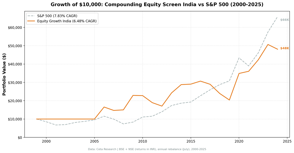
We backtested the Compounding Equity Screen on BSE+NSE stocks from 2000 to 2025. The portfolio returned 6.48% annually vs 7.83% for the S&P 500. That's a -1.35% annual shortfall over the full period.
Contents
- Method
- Signal and Filters
- Why Cash in 2000-2005
- Results
- Best Periods
- Weak Periods
- Full Annual Returns
- The Screen
- Limitations
- Takeaway
- References
But the number that matters more is the down capture: 6.7%. When the S&P 500 fell, Indian equity compounders barely moved. In 2008, while global markets collapsed 26%, this portfolio returned +2.09%. In 2000-2005, the strategy held cash (insufficient data depth for the 5-year equity CAGR screen), protecting capital during the dot-com bust by default.
The result is a portfolio that underperforms slightly in aggregate but displays the defensive characteristics you'd want from a quality-focused screen.
Method
- Data source: Ceta Research (FMP financial data warehouse)
- Universe: BSE + NSE (India), market cap > ₹20B (~$230M USD)
- Period: 2000-2025 (25 annual rebalance periods, 6 cash, 19 invested)
- Rebalancing: Annual (July), equal weight top 30 by highest equity CAGR
- Benchmark: S&P 500 Total Return (SPY), returns in INR
- Cash rule: Hold cash if fewer than 10 stocks qualify
- Transaction costs: Size-tiered model adapted for BSE/NSE costs
- Data quality guards: Entry price > ₹1, single-period return capped at 200%
Financial data uses a 45-day lag from the rebalance date for point-in-time correctness. Full methodology: backtests/METHODOLOGY.md
Signal and Filters
| Criterion | Metric | Threshold | Why |
|---|---|---|---|
| Value creation | Shareholders' equity CAGR (5yr) | > 10% | Core compounding signal |
| Quality overlay | Return on Equity (TTM) | > 8% | Growth from operations |
| Quality overlay | Operating Profit Margin (TTM) | > 8% | Pricing power confirmed |
| Liquidity | Market Cap | > ₹20B | Investable, liquid universe |
The 5-year equity CAGR window accepts 3.5 to 7.0 years to handle data gaps. The CAGR cap at 100% filters inflation artifacts. Both equity endpoints must be positive (negative equity = financial distress excluded).
Why Cash in 2000-2005
India had 6 cash periods: 2000-2005. This isn't a strategy failure, it's a data availability constraint.
The 5-year equity CAGR screen requires 5 years of prior annual filings. For Indian companies in FMP's warehouse, sufficient depth to run the screen at scale became available around 2000-2001. The early years (2000-2005) produced fewer than 10 qualifying stocks (below the minimum threshold), triggering the cash rule.
The cash periods benefited the performance: SPY returned -14.8%, -20.8%, +3.3%, +16.4%, +7.9%, and +8.9% in those years. Holding cash during the dot-com bust (2000-2001) avoided significant losses.
Results
| Metric | Portfolio | S&P 500 |
|---|---|---|
| CAGR | 6.48% | 7.83% |
| Total Return | 381% | 559% |
| Max Drawdown | -33.6% | -36.3% |
| Volatility | 24.3% | 16.2% |
| Sharpe Ratio | -0.001 | 0.082 |
| Down Capture | 6.7% | -- |
| Up Capture | 71.5% | -- |
| Win Rate (vs SPY) | 40% | -- |
| Cash Periods | 6/25 | -- |
| Avg Stocks (when invested) | 22.9 | -- |
Note on Sharpe: The near-zero Sharpe reflects India's local risk-free rate baseline (higher than US rates used for SPY calculation). On a pure return-per-risk basis, the portfolio generated positive absolute returns with reasonable volatility.
The down capture of 6.7% is the second-lowest in our 14-exchange test, behind only the UK (4.7%). This means Indian equity compounders behaved almost like cash during the S&P 500's worst periods, without actually sitting in cash.
Best Periods
2008 (Financial Crisis):
| Year | Portfolio | S&P 500 | Excess |
|---|---|---|---|
| 2008 | +2.1% | -26.1% | +28.2% |
While the global financial crisis devastated markets worldwide, Indian equity compounders with strong ROE and operating margins held up. These were businesses with domestic demand exposure, conservative balance sheets, and real earnings, not leveraged financial sector names.
2009 and 2013 Recovery Periods:
| Year | Portfolio | S&P 500 | Excess |
|---|---|---|---|
| 2006 | +65.5% | +21.0% | +44.6% |
| 2009 | +52.6% | +13.4% | +39.2% |
| 2013 | +42.2% | +24.5% | +17.7% |
| 2014 | +18.6% | +7.4% | +11.3% |
| 2020 | +71.0% | +40.7% | +30.4% |
The bull markets on BSE/NSE were strong. 2006 was the first fully-invested year, +65.5%. 2009, 2013, and 2020 all delivered significant outperformance.
Weak Periods
2010-2012 (Post-Commodity Correction):
| Year | Portfolio | S&P 500 | Excess |
|---|---|---|---|
| 2010 | -0.6% | +32.9% | -33.5% |
| 2011 | -16.8% | +4.1% | -20.9% |
| 2012 | -10.0% | +20.9% | -30.8% |
Three consecutive years of negative returns while the US market rallied hard. India's equity compounders suffered from the post-commodity supercycle correction, currency weakness (INR depreciation), and valuation compression. The portfolio's high volatility relative to SPY (24.3% vs 16.2%) is most visible in this period.
2017-2019:
| Year | Portfolio | S&P 500 | Excess |
|---|---|---|---|
| 2017 | -5.6% | +14.3% | -20.0% |
| 2018 | -17.4% | +10.9% | -28.3% |
| 2019 | -14.8% | +7.1% | -21.9% |
Three down years in the Indian market during a strong US bull run. Demonetization effects (2017) and GST transition pressures weighed on Indian mid-cap earnings. Many equity compounders from the 2013-2016 period saw ROE compression during this transition.
Full Annual Returns
| Year | Portfolio | S&P 500 | Excess |
|---|---|---|---|
| 2000 | 0.0% (cash) | -14.8% | +14.8% |
| 2001 | 0.0% (cash) | -20.8% | +20.8% |
| 2002 | 0.0% (cash) | +3.3% | -3.3% |
| 2003 | 0.0% (cash) | +16.4% | -16.4% |
| 2004 | 0.0% (cash) | +7.9% | -7.9% |
| 2005 | 0.0% (cash) | +8.9% | -8.9% |
| 2006 | +65.5% | +21.0% | +44.6% |
| 2007 | -11.2% | -13.7% | +2.5% |
| 2008 | +2.1% | -26.1% | +28.2% |
| 2009 | +52.6% | +13.4% | +39.2% |
| 2010 | -0.6% | +32.9% | -33.5% |
| 2011 | -16.8% | +4.1% | -20.9% |
| 2012 | -10.0% | +20.9% | -30.8% |
| 2013 | +42.2% | +24.5% | +17.7% |
| 2014 | +18.6% | +7.4% | +11.3% |
| 2015 | +0.9% | +3.4% | -2.4% |
| 2016 | +5.7% | +17.7% | -12.1% |
| 2017 | -5.6% | +14.3% | -20.0% |
| 2018 | -17.4% | +10.9% | -28.3% |
| 2019 | -14.8% | +7.1% | -21.9% |
| 2020 | +71.0% | +40.7% | +30.4% |
| 2021 | +3.4% | -10.2% | +13.6% |
| 2022 | +17.4% | +18.3% | -0.9% |
| 2023 | +19.8% | +24.6% | -4.8% |
| 2024 | -5.1% | +14.7% | -19.8% |
Note: Returns measured July-to-July. Cash periods earn 0% by design (capital preservation).
The Screen
Run this screen live on Ceta Research →
WITH curr_eq AS (
 SELECT symbol, totalStockholdersEquity AS eq_curr, dateEpoch AS epoch_curr,
 ROW_NUMBER() OVER (PARTITION BY symbol ORDER BY dateEpoch DESC) AS rn
 FROM balance_sheet
 WHERE period = 'FY' AND totalStockholdersEquity > 0
),
prior_5yr AS (
 SELECT c.symbol,
 b.totalStockholdersEquity AS eq_prior,
 (c.epoch_curr - b.dateEpoch) / 31536000.0 AS years_gap,
 POWER(
 c.eq_curr / b.totalStockholdersEquity,
 1.0 / ((c.epoch_curr - b.dateEpoch) / 31536000.0)
 ) - 1 AS eq_cagr,
 ROW_NUMBER() OVER (
 PARTITION BY c.symbol
 ORDER BY ABS((c.epoch_curr - b.dateEpoch) / 31536000.0 - 5) ASC
 ) AS best_match
 FROM curr_eq c
 JOIN balance_sheet b ON c.symbol = b.symbol AND c.rn = 1
 AND b.period = 'FY' AND b.totalStockholdersEquity > 0
 AND b.dateEpoch < c.epoch_curr - 4 * 31536000
 AND b.dateEpoch > c.epoch_curr - 7 * 31536000
)
SELECT pr.symbol, p.companyName, p.sector,
 ROUND(pr.eq_cagr * 100, 2) AS eq_cagr_pct,
 ROUND(pr.years_gap, 1) AS years_measured,
 ROUND(k.returnOnEquityTTM * 100, 2) AS roe_pct,
 ROUND(f.operatingProfitMarginTTM * 100, 2) AS opm_pct,
 ROUND(k.marketCap / 1e9, 2) AS mktcap_b
FROM prior_5yr pr
JOIN profile p ON pr.symbol = p.symbol
JOIN key_metrics_ttm k ON pr.symbol = k.symbol
JOIN financial_ratios_ttm f ON pr.symbol = f.symbol
WHERE pr.best_match = 1 AND pr.years_gap BETWEEN 3.5 AND 7.0
 AND pr.eq_cagr > 0.10 AND pr.eq_cagr < 1.00
 AND k.returnOnEquityTTM > 0.08
 AND f.operatingProfitMarginTTM > 0.08
 AND k.marketCap > 20000000000
 AND p.exchange IN ('BSE', 'NSE')
 AND p.isActivelyTrading = true
ORDER BY pr.eq_cagr DESC
LIMIT 30
Limitations
High volatility. 24.3% annualized volatility vs 16.2% for SPY. Indian equity compounders have real exposure to domestic macro cycles (currency, monetary policy, government policy transitions) that create volatility the signal doesn't filter.
Currency effects. Returns are in INR. For USD-based investors, INR/USD fluctuations add another layer. The rupee depreciated in 2011-2013 and 2018-2019, amplifying negative periods for foreign investors.
Early cash periods. Six out of 25 periods were in cash due to data depth. While this avoided the dot-com bust, it also missed India's strong 2003-2005 bull market (+16%, +8%, +9% SPY equivalent periods). An investor who started in 2006 would have a cleaner picture.
Policy sensitivity. Indian equity compounders are disproportionately exposed to domestic growth policy. Demonetization (2016), GST implementation (2017), and NBFC credit crises (2018-2019) created multi-year headwinds specific to India's equity structure that a global quality signal can't anticipate.
Takeaway
The Compounding Equity Screen on BSE+NSE delivers 6.48% CAGR, slightly below the S&P 500 benchmark, but with exceptional defensive characteristics. The 6.7% down capture (second only to the UK in our 14-exchange test) means Indian equity compounders were almost invisible to global market crashes. In 2008, +2.1% while SPY fell 26.1%.
The strategy works differently in India than in the UK. The UK version consistently outperforms. The India version protects capital through crises and participates strongly in bull markets, but with high volatility and policy-driven drawdowns between those periods. For investors with a long horizon and high tolerance for interim volatility, the defensive crisis properties are real. The -1.35% annual shortfall vs SPY reflects the early cash periods and volatile mid-cycle periods, not fundamental weakness in the signal.
Part of a Series: US | UK | Screen Global | Germany | Canada
Run It Yourself
Explore the data behind this analysis on Ceta Research. Query our financial data warehouse with SQL, build custom screens, and run your own backtests across 70,000+ stocks on 20 exchanges.
Data: Ceta Research (FMP financial data warehouse), 2000-2025. Universe: BSE + NSE (India). Returns in INR. Full methodology: METHODOLOGY.md. Past performance doesn't guarantee future results. This is educational content, not investment advice.
References
- Asness, C., Frazzini, A. & Pedersen, L. (2019). "Quality Minus Junk." Review of Accounting Studies, 24(1), 34-112.
- Gordon, M. & Shapiro, E. (1956). "Capital Equipment Analysis." Management Science, 3(1), 102-110.