Pairs Trading: How It Works and What 20 Years of Data Actually Shows

Most trading strategies bet on direction. Bull or bear, up or down. Pairs trading takes a different approach. It bets that two related stocks will snap back together after temporarily diverging. The market can go anywhere. What matters is the relationship between two specific stocks.
Contents
- Method
- What Is Pairs Trading?
- Correlation vs Cointegration
- The Academic Evidence
- What We Found: 2005-2024
- The Signal in Pictures
- The Benchmark Question
- Why Profitability Declined
- Across 12 Exchanges
- How Pairs Trading Works in Practice
- Stage 1: Screening (Playlist 2)
- Stage 2: Cointegration Testing (Playlist 3)
- Stage 3: Signal Generation (Playlist 4)
- Stage 4: Portfolio Construction (Playlists 5-6)
- When Pairs Trading Works
- When Pairs Trading Fails
- The Screens
- Limitations
- Takeaway
- References
Here's how it works, what 40 years of academic research shows, and what actually happened when we ran the same approach on 2005-2024 data across 12 exchanges.
Method
- Data source: Ceta Research (FMP financial data, 70K+ stocks)
- Universe: Top 30 stocks per sector by market cap per exchange
- Pair selection: Same sector, 252-day returns correlation > 0.70, top 20 pairs
- Entry signal: |z-score| > 1.5 at year-end (formation year)
- Return model: Equal-dollar pairs return =
-sign(z) × (Return_A - Return_B) / 2 - Rebalancing: Annual, 2005-2024
- Costs: 4 one-way legs per pair (open + close × 2 stocks)
- Academic reference: Gatev, Goetzmann & Rouwenhorst (2006), Review of Financial Studies
What Is Pairs Trading?
Pairs trading is a market-neutral strategy. You hold a long position in one stock and a short position in another, simultaneously. The two stocks are chosen because they historically move together. When they temporarily diverge, you bet on convergence.
Concrete example: Exxon (XOM) and Chevron (CVX) are both large-cap oil companies. Their stock prices are driven by similar factors: oil prices, energy demand, refinery margins, regulatory changes. Over long stretches, they tend to move in tandem.
But they don't move in lockstep every day. Earnings surprises, analyst upgrades, company-specific news all create temporary gaps. One stock drifts higher while the other lags. Pairs trading bets that gap will close.
The mechanic: if XOM drops 5% relative to CVX with no fundamental reason, you buy XOM and short CVX. When the spread normalizes, you close both positions. Your profit comes from the convergence, not from either stock going up or down in absolute terms.
This makes pairs trading market-neutral. If the entire energy sector crashes 20%, both your long and short positions lose value. But the loss on one is offset by the gain on the other. What matters is the relative performance, not the absolute direction.
Correlation vs Cointegration
Most people start with correlation. Two stocks with high correlation (above 0.80 over the past year) seem like good pairs candidates. That's a reasonable first filter, but it's incomplete.
Correlation measures whether two stocks move in the same direction. If XOM goes up 2% on days when CVX goes up 1.5%, they're positively correlated. But correlation doesn't tell you whether the spread between them is stationary, whether it tends to return to a mean.
Cointegration is the stronger requirement. Two stocks are cointegrated if some linear combination of their prices is stationary (mean-reverting). You can have two stocks with 0.90 correlation that aren't cointegrated. Their prices might drift apart permanently even though daily returns look similar.
Think of it like two friends walking their dogs. Correlation means both dogs tend to walk in the same direction. Cointegration means the dogs are on leashes, so even if they wander apart briefly, they snap back together. The leash length determines how far they can diverge.
For pairs trading, cointegration is what matters. Correlation is the first filter. Cointegration is the validation. We cover the statistical tests (Engle-Granger, ADF) in playlist 3.
The Academic Evidence
The foundational study is Gatev, Goetzmann and Rouwenhorst (2006), published in the Review of Financial Studies. They tested a simple pairs trading strategy on US equities from 1962 to 2002.
Their approach: form pairs based on minimum distance (sum of squared deviations of normalized prices) during a 12-month formation period. Open trades when pairs diverge by 2 standard deviations. Close when they converge or after 6 months.
Results (Gatev et al., 2006, pre-cost): - Average excess return: ~11% per year - Pairs converged ~80% of the time within the 6-month trading period - Strategy was profitable in 31 out of 40 years tested - Risk-adjusted returns were significant even after controlling for Fama-French factors
But that was 2002. What happened after?
Do and Faff (2010) extended the analysis to 2008. They found that pairs trading profitability declined after 2002. Their explanation: increased hedge fund activity and algorithmic trading compressed the arbitrage opportunity. More capital chasing the same mispricings meant smaller returns per trade.
Do and Faff (2012) followed up showing transaction costs further eroded profitability. After accounting for bid-ask spreads and borrowing costs, net returns were much lower than the gross figures in Gatev et al.
What We Found: 2005-2024
We ran a correlation-based pairs strategy on US stocks (NYSE + NASDAQ + AMEX) from 2005 to 2024. Same basic approach as Gatev et al., adapted for annual rebalance and z-score entry signals.
US results (NYSE + NASDAQ + AMEX):
| Metric | Value |
|---|---|
| CAGR (2005-2024) | 0.33% |
| vs SPY (10.01%) | -9.68% |
| Sharpe ratio | -0.407 |
| Max drawdown | -12.99% |
| Portfolio volatility | 4.10% |
| Cash periods (0 return) | 5/20 years (25%) |
| Avg active pairs | 5.2 |
| Beta to SPY | 0.10 |
The headline is 0.33% CAGR against SPY's 10.01%. That's a large gap. But the context matters.
This is a market-neutral strategy. Comparing it to SPY is measuring opportunity cost, not apples-to-apples. The right benchmark for a market-neutral strategy is the risk-free rate, not equities. Over this period, T-bills averaged roughly 2% annually. Against that benchmark, 0.33% still underperforms.
The volatility difference is notable: 4.10% for the pairs portfolio vs ~17% for SPY. The strategy ties up capital in offsetting positions and earns close to nothing on it, with much lower variance. That's not the same as losing money in the way a directional trade does.
Annual returns:
| Year | Pairs | SPY | Excess |
|---|---|---|---|
| 2005 | -8.8% | +7.2% | -16.0% |
| 2006 | +1.0% | +13.7% | -12.7% |
| 2007 | +0.4% | +5.3% | -4.9% |
| 2008 | -3.5% | -36.2% | +32.7% |
| 2009 | +5.3% | +22.7% | -17.4% |
| 2010 | 0% (cash) | +13.1% | -13.1% |
| 2011 | 0% (cash) | +2.5% | -2.5% |
| 2012 | +2.6% | +14.2% | -11.6% |
| 2013 | -0.7% | +29.0% | -29.7% |
| 2014 | -1.8% | +14.6% | -16.3% |
| 2015 | -6.6% | +1.3% | -7.8% |
| 2016 | -0.6% | +14.5% | -15.0% |
| 2017 | 0% (cash) | +21.6% | -21.6% |
| 2018 | -0.4% | -5.3% | +4.9% |
| 2019 | +1.4% | +31.1% | -29.7% |
| 2020 | +9.2% | +17.2% | -8.0% |
| 2021 | 0% (cash) | +30.5% | -30.5% |
| 2022 | 0% (cash) | -19.0% | +19.0% |
| 2023 | +7.1% | +26.0% | -18.9% |
| 2024 | +3.5% | +25.6% | -22.1% |
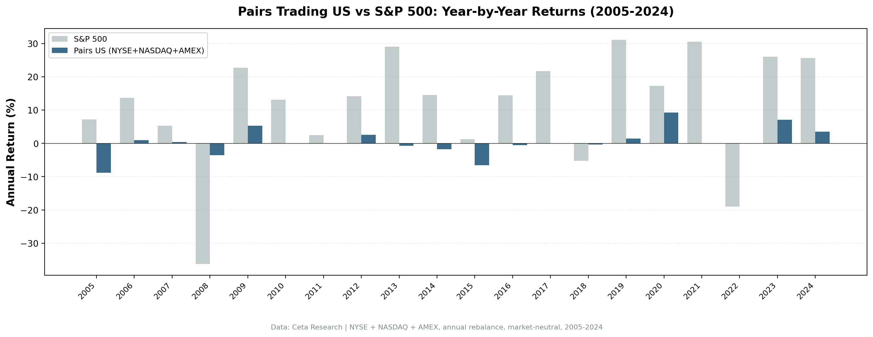
2008 is the defining year. The S&P 500 fell 36.2%. The pairs portfolio fell 3.5%. That's +32.7% excess performance. The pairs strategy did exactly what market-neutral is supposed to do in a crisis: offset long and short positions, collect the spread, stay largely insulated from the directional collapse.
Five cash years. The strategy sat out 2010, 2011, 2017, 2021, and 2022 entirely (fewer than 3 active pairs with |z| > 1.5). In a bull market like 2017 (+21.6% SPY) or 2021 (+30.5%), being in cash is expensive. In 2022 (-19% SPY), being in cash was +19%.
Win rate vs SPY: 15%. The strategy outperformed SPY in 3 of 20 years (2008, 2018, 2022). All three were years SPY fell.
The Signal in Pictures

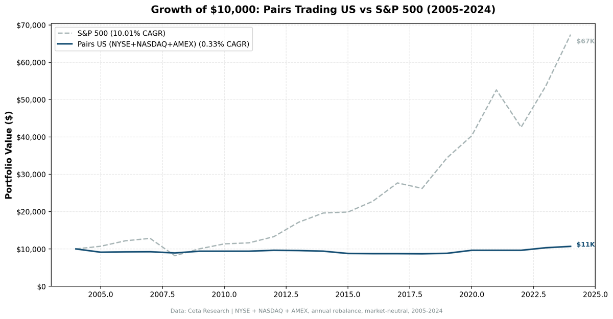
$10,000 in the pairs portfolio grew to $10,671 over 20 years. SPY grew to $65,274. The gap is mostly opportunity cost, capital sitting in offsetting positions earning near-zero.
The strategy's one consistent feature: it didn't fall in 2008. In most other years, SPY's upside momentum was simply too strong to offset.
The Benchmark Question
One thing to get straight before comparing these numbers to anything: SPY isn't the right benchmark for a market-neutral strategy.
SPY measures equity market returns. Pairs trading doesn't take equity market risk. Beta is 0.10. The strategy is holding equal-dollar longs and shorts simultaneously. Its risk profile is nothing like owning the S&P 500.
The appropriate benchmark is the risk-free rate. T-bills averaged approximately 2% over 2005-2024. Against T-bills, the pairs portfolio (0.33% CAGR) still underperforms by about 1.7% annually.
So the honest summary: the strategy earns less than T-bills with 4% volatility, and earns meaningfully less than SPY. But it also has much lower volatility, nearly zero equity beta, and its best years were the equity market's worst years.
That profile is different from both stocks and bonds. It's not obviously attractive as a standalone strategy in this period, but it has a role in a portfolio where low correlation to equities has value.
Why Profitability Declined
The academic explanation (Do & Faff 2010) is crowding. Pairs trading became well-known in the late 1990s and early 2000s. As more capital chased the same mispricings:
- Spreads at entry got smaller (more competition to buy the cheap leg)
- Spreads at exit got larger (more competition to close)
- Net profitability per trade compressed
The Gatev et al. pre-2002 data showed 11% excess returns. Our 2005-2024 data shows 0.33% CAGR. The trend is directional: each decade, returns have declined.
There's also a signal problem with annual rebalancing. Real pairs traders check spreads daily, not annually. An annual z-score check misses most of the intra-year pairs activity. The backtest likely understates what a daily implementation would produce (or overestimates, hard to say without testing it).
Across 12 Exchanges
We ran the same strategy on 12 exchanges globally. Results confirmed the pattern: near-zero nominal returns everywhere.
| Exchange | CAGR | Sharpe | Cash% |
|---|---|---|---|
| UK (LSE) | 1.83% | -0.201 | 65% |
| South Africa (JNB) | 1.57% | -0.777 | 15% |
| India (BSE+NSE) | 0.72% | -1.793 | 75% |
| Japan (JPX) | 0.61% | +0.141 | 5% |
| US (NYSE+NASDAQ+AMEX) | 0.33% | -0.407 | 25% |
| China (SHZ+SHH) | 0.23% | -0.570 | 40% |
| Hong Kong | 0.02% | -0.767 | 40% |
| Canada (TSX) | -0.05% | -0.668 | 25% |
| Sweden (STO) | -0.25% | -0.393 | 40% |
| Germany (XETRA) | -0.83% | -1.184 | 70% |
| Korea (KSC) | -0.90% | -0.976 | 45% |
| Taiwan (TAI+TWO) | -1.85% | -0.490 | 55% |
Japan stands out: the only market with a positive Sharpe (+0.141) and only 1 cash year out of 20. China and India results are theoretical, short-selling restrictions make the strategy difficult to implement there in practice.
We cover the Japan results in depth in the regional blog and do a full 12-exchange comparison here.
How Pairs Trading Works in Practice
The full workflow has four stages. Each gets its own playlist in this series.
Stage 1: Screening (Playlist 2)
Start with a universe (all US stocks > $1B market cap). Compute pairwise correlations within sectors. Filter for pairs with correlation above 0.70 over the past 252 trading days. Pre-filtering by sector is critical, with 2,000+ stocks, you have millions of potential pairs. Same sector cuts that to manageable numbers.
Stage 2: Cointegration Testing (Playlist 3)
Take the top correlated pairs. Run Engle-Granger cointegration tests: regress log-price A on log-price B to get the hedge ratio, compute the spread residual, run an ADF test. If the spread is stationary (p < 0.05), the pair is cointegrated.
Also compute the half-life of mean reversion. A half-life of 10-60 days is practical. Below 5 days means signal moves faster than you can trade. Above 120 days means you're waiting too long for convergence.
Stage 3: Signal Generation (Playlist 4)
For validated pairs, construct the spread and normalize it into a z-score. Entry when |z| > 1.5-2.0. Exit when |z| < 0.5.
The hedge ratio determines how many shares of each stock to hold. Both fixed OLS (computed once at formation) and rolling OLS (updated daily) have trade-offs. Fixed is simpler but can drift as the relationship changes.
Stage 4: Portfolio Construction (Playlists 5-6)
Run the strategy across multiple pairs simultaneously. Manage portfolio-level risk: sector concentration, net exposure, position sizing. Replace pairs when cointegration breaks down.
When Pairs Trading Works
Market stress. When sector-level factors dominate stock-specific factors, related stocks tend to diverge temporarily and converge. The 2008 data is the clearest example.
Stable macro environments. Low volatility, high intra-sector correlation periods (like 2004-2007) create more entry opportunities.
Markets with structural cross-shareholding. Japan's keiretsu network creates stable long-term relationships between related companies. That's likely why JPX shows higher investment rates (5% cash) than other exchanges.
When Pairs Trading Fails
Structural breaks. If one company in a pair changes (acquisition, business pivot, regulatory change), the historical relationship breaks down. The spread diverges and doesn't come back.
Regime changes. COVID 2020 disrupted correlations across many sectors. The 2008 crisis itself, while good for pairs returns, broke many long-standing correlations.
Crowding. As pairs trading became popular in the late 1990s, returns declined. More capital chasing the same mispricings means smaller profits per trade.
Annual rebalancing. Annual z-score checks miss most intra-year opportunities. Daily monitoring would produce different (likely higher) gross returns, but also much higher transaction costs.
The Screens
Current high-correlation pairs in the US market, by sector:
WITH sector_map AS (
 SELECT DISTINCT symbol, sector
 FROM profile
 WHERE exchange IN ('NYSE', 'NASDAQ', 'AMEX')
 AND sector IS NOT NULL
 AND isActivelyTrading = true
),
large_caps AS (
 SELECT km.symbol, sm.sector
 FROM key_metrics km
 JOIN sector_map sm ON km.symbol = sm.symbol
 WHERE km.period = 'FY'
 AND km.marketCap > 1000000000
 QUALIFY ROW_NUMBER() OVER (PARTITION BY km.symbol ORDER BY km.dateEpoch DESC) = 1
),
daily_ret AS (
 SELECT eod.symbol, CAST(eod.date AS DATE) AS trade_date,
 (eod.adjClose - LAG(eod.adjClose) OVER (PARTITION BY eod.symbol ORDER BY eod.date))
 / NULLIF(LAG(eod.adjClose) OVER (PARTITION BY eod.symbol ORDER BY eod.date), 0) AS ret
 FROM stock_eod eod
 JOIN large_caps lc ON eod.symbol = lc.symbol
 WHERE eod.date >= (CURRENT_DATE - INTERVAL '365 days')
)
SELECT a.symbol AS symbol_a, b.symbol AS symbol_b, la.sector,
 ROUND(CORR(a.ret, b.ret), 4) AS correlation,
 COUNT(*) AS common_days
FROM daily_ret a
JOIN daily_ret b ON a.trade_date = b.trade_date AND a.symbol < b.symbol
JOIN large_caps la ON a.symbol = la.symbol
JOIN large_caps lb ON b.symbol = lb.symbol
WHERE a.ret IS NOT NULL AND b.ret IS NOT NULL AND la.sector = lb.sector
GROUP BY a.symbol, b.symbol, la.sector
HAVING COUNT(*) >= 200
 AND CORR(a.ret, b.ret) >= 0.70
ORDER BY correlation DESC
LIMIT 20
Limitations
Survivorship bias. This backtest uses currently active stocks only. Companies that went bankrupt or were acquired are excluded. This slightly biases results upward, since the excluded companies likely performed worse. The effect is modest in a market-neutral strategy, but it's not zero.
Short-selling constraints. China (SHZ+SHH) and India (BSE+NSE) results are theoretical. Both markets have significant restrictions on short-selling. The pairs strategy can't be run there as described without modifications.
Annual rebalancing. A daily implementation would see more pairs, different entry points, and much higher transaction costs. The backtest represents a stylized annual version, not a live trading system.
Model risk. Correlation threshold (0.70), z-score entry (1.5), minimum pairs (3), max pairs (20), all parameter choices affect results. The parameters weren't optimized on this dataset; they were set based on the Gatev et al. approach.
Takeaway
Pairs trading is a market-neutral strategy that exploits temporary divergences between related stocks. The theory is sound. The 1962-2002 data showed 11% excess returns. The 2005-2024 data shows near-zero nominal returns.
The strategy isn't dead. It still does what it's supposed to do in the worst equity markets. In 2008, +32.7% excess. In 2022, the cash position avoided a -19% SPY year. The problem is that these defensive wins are rare and most years the strategy earns less than T-bills.
Whether that profile is useful depends on what else is in your portfolio. Low equity correlation has value. But 0.33% CAGR against T-bills at 2% is a hard sell as a standalone strategy.
The next five playlists walk through each stage of the pairs trading workflow in detail: pair screening, cointegration testing, signal generation, and a full 20-year backtest.
References
- Gatev, E., Goetzmann, W. & Rouwenhorst, K. (2006). "Pairs Trading: Performance of a Relative-Value Arbitrage Rule." Review of Financial Studies, 19(3), 797-827.
- Do, B. & Faff, R. (2010). "Does Simple Pairs Trading Still Work?" Financial Analysts Journal, 66(4), 83-95.
- Do, B. & Faff, R. (2012). "Are Pairs Trading Profits Robust to Trading Costs?" Journal of Financial Research, 35(2), 261-287.
- Krauss, C. (2017). "Statistical Arbitrage Pairs Trading Strategies: Review and Outlook." Journal of Economic Surveys, 31(2), 513-545.
- Vidyamurthy, G. (2004). Pairs Trading: Quantitative Methods and Analysis. John Wiley & Sons.
- Engle, R. & Granger, C. (1987). "Co-Integration and Error Correction: Representation, Estimation, and Testing." Econometrica, 55(2), 251-276.
Part of a Series: Global | Backtest Global Results | Japan | US | US | US | Japan
Run It Yourself
Explore the data behind this analysis on Ceta Research. Query our financial data warehouse with SQL, build custom screens, and run your own backtests across 70,000+ stocks on 20 exchanges.
Data: Ceta Research, FMP warehouse, stock_eod + profile + key_metrics tables Note: Past performance doesn't guarantee future results. This is educational content, not investment advice. Backtest code: github.com/ceta-research/backtests