Cointegration Testing for Pairs Trading: Why 80% of Correlated Pairs

We screened 3,701 US large-cap stocks down to 2,579 highly correlated candidate pairs. Then we ran statistical cointegration tests on all of them. Only 516 passed (20.0%). Here's what that means, why it matters, and what the 80% failure rate tells you about pairs trading in practice.
Contents
- The Core Distinction
- Method
- The Engle-Granger Two-Step Method
- Step 1: Estimate the Hedge Ratio
- Step 2: Test the Residuals for Stationarity
- Half-Life of Mean Reversion
- Results
- Overall Pass Rate
- By Sector
- Lower Correlation Predicts Higher Pass Rate
- Half-Life Distribution
- Why Pairs Fail Cointegration Testing
- Trending Spread (Most Common)
- Structural Breaks
- High Correlation from a Single Event
- Spread Construction in SQL
- Run It Yourself
- Limitations
- Part of a Series

The Core Distinction
Correlation tells you two stocks tend to move in the same direction on the same day. Cointegration tells you the gap between them is stable over time. These sound similar. They're not.
Two stocks can move in the same direction every day and still drift apart permanently. Think of two hikers walking the same trail in the same direction. Perfectly correlated movement, but the distance between them grows without limit. You can't trade that gap.
Cointegrated stocks are different. The gap between them fluctuates, but it snaps back. Think of two hikers connected by a bungee cord. They wander apart, the cord stretches, and they're pulled back together. That's tradeable.
Engle and Granger won the Nobel Prize in 2003 for formalizing this distinction. Their 1987 paper laid out the two-step procedure that remains the standard test for pairwise cointegration.
Method
- Data: Ceta Research (FMP financial data warehouse)
- Universe: US stocks > $1B market cap, 3,701 stocks
- Input: 2,579 candidate pairs from correlation screening (corr ≥ 0.80, same sector, market cap ratio < 5x)
- Price data:
stock_eodtable (adjClose), lookback: 252 trading days - Statistical test: Augmented Dickey-Fuller (ADF) on Engle-Granger residuals
- Pass criteria: ADF p-value < 0.05 AND half-life 5-120 trading days
The Engle-Granger Two-Step Method
Step 1: Estimate the Hedge Ratio
Run an OLS regression of one price series on the other:
Price_A(t) = alpha + beta * Price_B(t) + epsilon(t)
The coefficient beta is the hedge ratio. For a pair like XOM and CVX, if beta is 0.62, the spread is:
spread(t) = Price_XOM(t) - 0.62 * Price_CVX(t)
The hedge ratio means: for every $1 of XOM you hold long, you hold $0.62 of CVX short. This minimizes the variance of the spread.
Using a fixed 1:1 ratio (just Price_A minus Price_B) only works when both stocks have similar price levels and volatility. The OLS-derived ratio accounts for the actual relationship.
Step 2: Test the Residuals for Stationarity
The residuals from Step 1 (the spread) should be stationary if the pair is cointegrated. We test this with the Augmented Dickey-Fuller test.
The ADF test checks the null hypothesis that the spread has a unit root (it's a random walk). If we reject the null (p-value < 0.05), the spread is stationary and the pair is cointegrated.
from statsmodels.tsa.stattools import adfuller

result = adfuller(spread, maxlag=20, autolag='AIC')
adf_stat = result[0]
p_value = result[1]
Critical values at 252 observations:
| Significance | Critical Value |
|---|---|
| 1% | -3.46 |
| 5% | -2.87 |
| 10% | -2.57 |
If the test statistic is more negative than the critical value, reject the null. The spread is stationary.
Half-Life of Mean Reversion
A pair can be cointegrated but revert so slowly it's untradeable. The half-life tells you how long the spread takes to revert halfway to its mean.
It comes from fitting an AR(1) model to the spread:
spread(t) - spread(t-1) = phi * spread(t-1) + noise
half_life = -log(2) / log(1 + phi)
Where phi is the AR(1) coefficient. A negative phi means the spread reverts to the mean. The more negative, the faster.
Practical ranges: - Half-life < 5 days: Too fast. Transaction costs eat the profit. - Half-life 5-30 days: Sweet spot for active pairs trading. - Half-life 30-120 days: Viable for patient, low-turnover strategies. - Half-life > 120 days: Capital locked up too long. Structural break risk is high.
We filter for half-life between 5 and 120 days.
Results
Overall Pass Rate
Starting from 2,579 candidate pairs (correlation ≥ 0.80, same sector, similar market cap):
| Filter Stage | Pairs | Pass Rate |
|---|---|---|
| Screening candidates (corr ≥ 0.80) | 2,579 | 100% |
| ADF p-value < 0.05 | 516 | 20.0% |
| ADF p-value < 0.01 | 198 | 7.7% |
All 516 pairs that passed ADF also passed the half-life filter (5-120 days). None had half-lives above 60 days.
The pass rate is 20.0%. Four in five highly correlated pairs have no stable spread to trade.
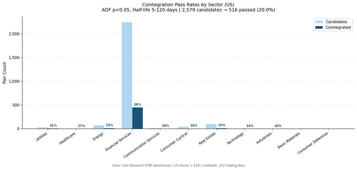
By Sector
| Sector | Candidates | Cointegrated | Pass Rate |
|---|---|---|---|
| Utilities | 35 | 11 | 31.4% |
| Healthcare | 11 | 3 | 27.3% |
| Energy | 79 | 18 | 22.8% |
| Financial Services | 2,249 | 453 | 20.1% |
| Communication Services | 20 | 4 | 20.0% |
| Consumer Cyclical | 49 | 8 | 16.3% |
| Real Estate | 106 | 16 | 15.1% |
| Technology | 14 | 2 | 14.3% |
| Industrials | 10 | 1 | 10.0% |
| Basic Materials | 4 | 0 | 0% |
| Consumer Defensive | 2 | 0 | 0% |
Utilities leads at 31.4%, driven by common regulatory and interest-rate exposure across all utility stocks. Energy is second at 22.8%, driven by commodity price sensitivity. Technology trails at 14.3%: each company has a unique growth trajectory that creates trending spreads.
Healthcare's 27.3% looks high, but 3 of 11 is a thin sample. Take it as directional.
Lower Correlation Predicts Higher Pass Rate
This is the counterintuitive finding. You'd expect higher-correlated pairs to be better cointegrated. The data says the opposite:
| Correlation Range | Candidates | Cointegrated | Pass Rate |
|---|---|---|---|
| 0.80-0.85 | 2,086 | 436 | 20.9% |
| 0.85-0.90 | 391 | 64 | 16.4% |
| 0.90-0.95 | 36 | 5 | 13.9% |
| 0.95-1.00 | 66 | 11 | 16.7% |
The 0.95-1.00 bucket contains share-class pairs (GOOG/GOOGL), corporate restructuring artifacts, and ETFs tracking the same index. These have near-perfect correlation but tight, low-volatility spreads that often pass ADF because there's almost no spread to test. The 0.80-0.85 bucket contains pairs with a real economic relationship that aren't perfectly synchronized, which is the signal you want.
Half-Life Distribution
All 516 cointegrated pairs have half-lives between 5.1 and 59.8 days. The distribution is heavily concentrated in the 15-20 day range.
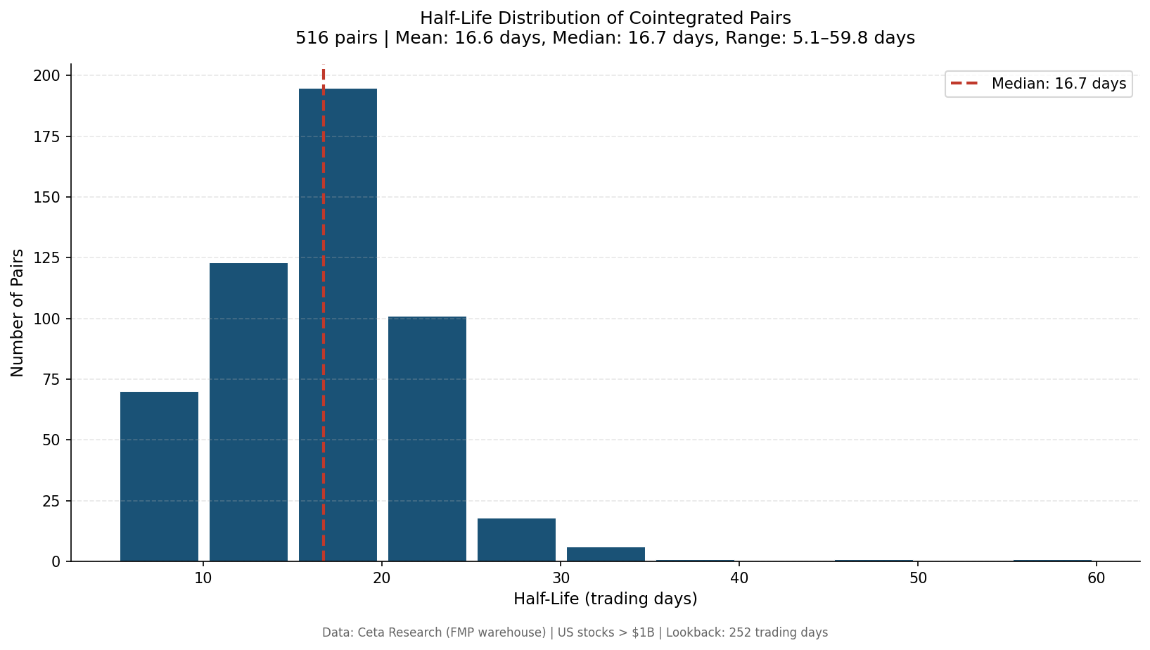
| Half-Life Range | Count | Percentage |
|---|---|---|
| 5-15 days | 193 | 37.4% |
| 15-30 days | 314 | 60.9% |
| 30-60 days | 9 | 1.7% |
| 60+ days | 0 | 0.0% |
The median is 16.7 days. Most cointegrated pairs revert within 3-4 weeks. This is the dominant regime in the US large-cap universe.
No pairs exceeded 60 days. The 120-day upper bound in the filter never bound. US large-cap pairs either revert fast or don't revert at all.
Why Pairs Fail Cointegration Testing
Trending Spread (Most Common)
Two stocks are correlated because they both participated in the same sector rally. But one grew faster than the other, so the spread trends upward. The ADF test correctly identifies this as non-stationary.
A fast-growing SaaS company paired with a mature tech firm: both in Technology, both rose in 2023-2024. But the growth stock appreciated 80% while the mature firm appreciated 30%. Their spread trends, and no hedge ratio fixes it.
Structural Breaks
A pair that was cointegrated for three years suddenly breaks apart. Acquisitions, CEO changes, regulatory shifts, or a fundamental change in business model can all cause this.
The ADF test on the full period might still show cointegration because the first three years dominate the statistics. But the relationship is gone. This is why re-testing periodically matters.
High Correlation from a Single Event
Some pairs have high correlation because they both responded to the same macro event (COVID, rate spike, earnings season). That event-driven correlation doesn't create a stable long-run spread.
Spread Construction in SQL
Once you have the hedge ratio from Python, spread construction and rolling statistics run entirely in SQL:
WITH pair_prices AS (
 SELECT
 a.trade_date,
 a.adjClose AS price_a,
 b.adjClose AS price_b,
 a.adjClose - 0.62 * b.adjClose AS spread
 FROM stock_eod a
 JOIN stock_eod b ON a.trade_date = b.trade_date
 WHERE a.symbol = 'XOM' AND b.symbol = 'CVX'
 AND a.trade_date >= '2024-01-01'
 QUALIFY ROW_NUMBER() OVER (PARTITION BY a.trade_date ORDER BY a.date DESC) = 1
)
SELECT
 trade_date,
 spread,
 AVG(spread) OVER (ORDER BY trade_date ROWS BETWEEN 59 PRECEDING AND CURRENT ROW) AS spread_mean_60,
 STDDEV(spread) OVER (ORDER BY trade_date ROWS BETWEEN 59 PRECEDING AND CURRENT ROW) AS spread_std_60,
 (spread - AVG(spread) OVER (ORDER BY trade_date ROWS BETWEEN 59 PRECEDING AND CURRENT ROW))
 / NULLIF(STDDEV(spread) OVER (ORDER BY trade_date ROWS BETWEEN 59 PRECEDING AND CURRENT ROW), 0) AS z_score
FROM pair_prices
ORDER BY trade_date
The z-score is the trading signal. When it exceeds +/- 2, the spread has deviated from its mean. Series 4 (z-score signals) covers the entry and exit rules in detail.
Part of a Series: Global | Backtest Global Results | Japan | Fundamentals | US | US | Japan
Run It Yourself
The cointegration pipeline is in backtests/pairs-cointegration/. It takes the candidate pairs from screening as input:
# Run cointegration test on all 2,579 candidate pairs
python3 pairs-cointegration/backtest.py \
 --input./ts-content-creator/content/_ready/pairs-02-screening/results/candidate_pairs.csv \
 --output results/cointegrated_pairs.csv \
 --verbose

# Screen current pairs for extended z-scores
python3 pairs-cointegration/screen.py --min-zscore 1.5
View the current cointegrated pairs and their spreads on Ceta Research:
View the XOM/CVX spread construction SQL on Ceta Research →
Limitations
252-day lookback is arbitrary. A longer lookback (504 or 756 days) might change which pairs pass. Relationships that look stable over one year may be unstable over two. We used 252 days because it's the industry standard for formation periods, but the choice affects results.
US large-cap only. The 20% pass rate applies to US stocks above $1B market cap. Small-cap pairs, international pairs, or sector-focused universes would give different results.
In-sample only. Finding cointegration on historical data doesn't guarantee it persists. The standard approach is to test on a training window and validate on a holdout period. We haven't done that here.
p-value thresholds are conventional, not magical. Using 0.05 vs 0.10 changes the pass count by roughly 50%. The 5% threshold is the convention from the statistics literature. It's not the only valid choice.
Structural breaks aren't handled. The standard ADF test assumes the relationship is stable across the full lookback window. If a company was acquired midway through the window, the test results are unreliable.
Pairs need periodic re-testing. Cointegration isn't permanent. Any production system needs monthly or quarterly re-testing and the ability to exit positions when relationships break down.
Part of a Series
- Pairs Trading Fundamentals. Theory and academic background
- Candidate Screening, 2,579 candidate pairs from 884,000 tests
- Cointegration Testing ← You are here
- Z-Score Signals. Entry and exit rules
- Backtest Results. Does it work? (Spoiler: barely)
- Multi-Pair Portfolio. Diversification across pairs
Run It Yourself
Explore the data behind this analysis on Ceta Research. Query our financial data warehouse with SQL, build custom screens, and run your own backtests across 70,000+ stocks on 20 exchanges.
Data: Ceta Research (FMP financial data warehouse), US stocks > $1B market cap, 252-day lookback ending Feb 2026. Full methodology: backtests/METHODOLOGY.md