52-Week Low Quality: 24-Year India Backtest (NSE)

India's result is worse than it looks: 3.62% CAGR over 24 years on NSE. Compare that to the Sensex, which returned 14.48% annually over the same period. The strategy trailed the local benchmark by -10.86% per year. The Sharpe ratio is -0.114. The strategy generated fewer returns with more risk than just holding the index. Here's what happened and why.

Contents

1. Method
2. What We Found
3. Year-by-Year
4. What the Data Is Telling You
5. Run It Yourself
6. Limitations

Data: FMP financial data warehouse, 2000–2025. Updated March 2026.

Method

Data source: Ceta Research (FMP financial data warehouse) Universe: NSE, market cap > ₹500M (~$6M USD local threshold) Period: 2002-2025 (95 quarters) Rebalancing: Quarterly (January, April, July, October), equal weight Max stocks: 30, minimum 5 to deploy capital Benchmark: BSE Sensex (local currency) Cash rule: Hold cash if fewer than 5 stocks qualify Transaction costs: 0.1% per trade (one-way) Filing lag: 45-day lag on all fundamental data Execution: Next-day close (market-on-close)

Full methodology: backtests/METHODOLOGY.md

What We Found

The Sharpe of -0.114 is the headline number. Negative means the strategy underperformed the risk-free rate after accounting for volatility. The Sensex's Sharpe over the same period is 0.341. This strategy took on 25.25% annualized volatility, deeper drawdowns than the Sensex (-55.06% vs -51.34%), and underperformed by 10.86% annually.

The up-capture of 54.25% means it captures just over half the Sensex's gains. When the Sensex gains 30%, this typically gains 16%. That asymmetry, sustained over 24 years, creates the massive terminal wealth gap: ₹1 lakh invested grew to ₹2.33 lakh in the strategy vs ₹24.84 lakh in the Sensex.

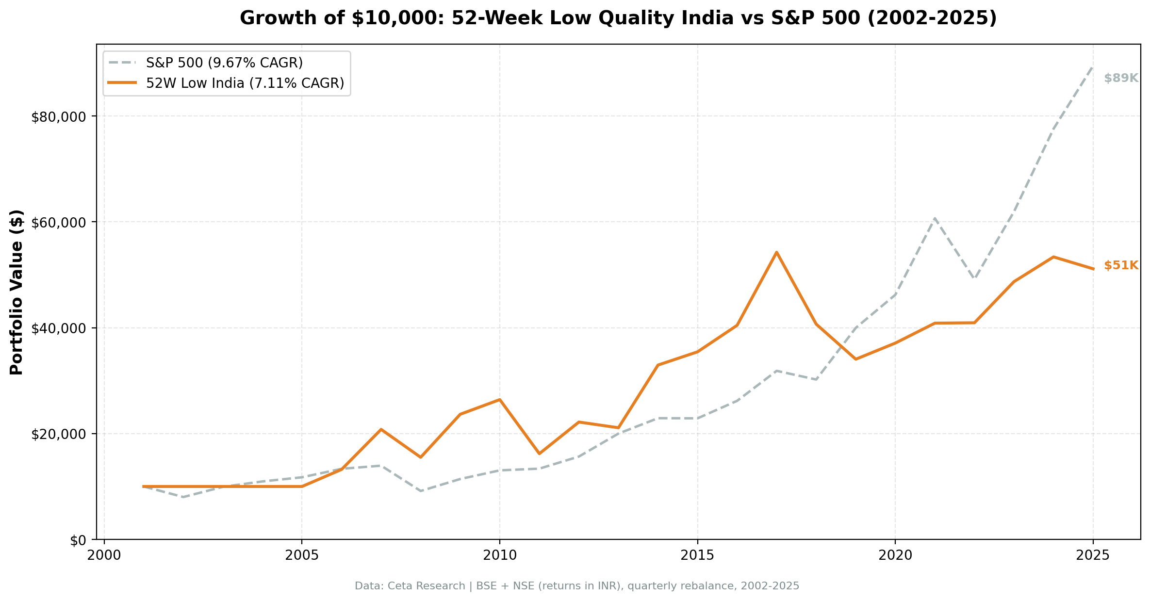
$10k invested in January 2002. India portfolio (blue) vs Sensex (grey) by December 2025.

Year-by-Year

The range here is extreme. 2014: +42.90% when the Sensex returned +33.51%. 2008: -30.67% when the Sensex lost -51.34%. 2015: +7.69% when the Sensex lost -8.12% (one of the few notable protection years). 2018: -18.77% when the Sensex gained +6.15%. 2019: -10.83% when the Sensex gained +15.98%. 2020: -3.46% when the Sensex gained +15.74%. These aren't modest deviations. The strategy swings against the benchmark in both directions, and five years out of the last eight (2016-2025) showed negative excess return.

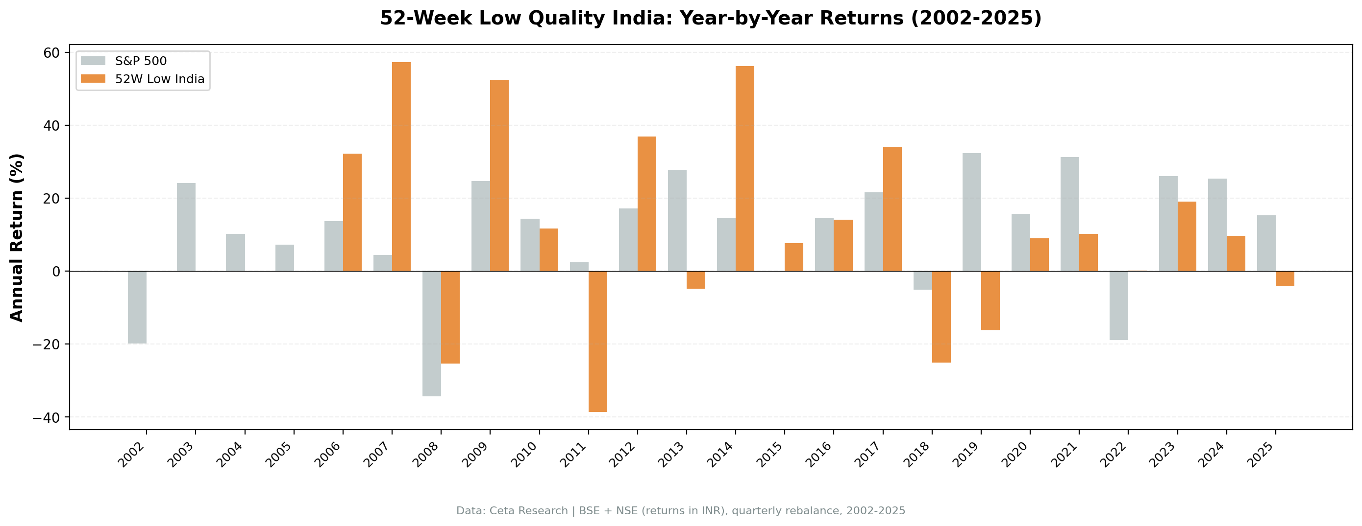
Year-by-year comparison. The large positive spikes (2007, 2014) are matched by significant negative years (2011, 2018, 2019). The variance is the story.

What the Data Is Telling You

The 32 cash periods (roughly eight full years of inactivity) are the starting point. India's NSE universe took time to develop enough qualifying stocks. In the early 2000s, fewer companies met both the proximity-to-52-week-low threshold and the Piotroski F-score >= 7 quality bar. The strategy sat in cash for the first five years of the backtest (2002-2006). NSE's structural maturation through the mid-2000s is the cause, not a parameter choice. During those early cash years, the Sensex returned +79%, +11%, +41%, and +48% in 2003-2006. That's opportunity cost the strategy can never recover.

When the strategy fires, the quality screen shows some value. The 2014 return of +42.90% beat the Sensex by 9.39 percentage points. 2015-2017 were three consecutive years of outperformance: +15.81%, +14.83%, and +11.48% excess. In 2008, the strategy lost -30.67% vs the Sensex's -51.34%, a +20.67% edge during the worst year of the test period.

But the wins don't compensate for the misses. The strategy was in cash for 2003 (Sensex +79%), 2004 (+11%), 2005 (+41%), 2006 (+48%). That's five years of India's strongest bull run, all in cash. And the late-period results are brutal: 2018 (-18.77% vs Sensex +6.15%), 2019 (-10.83% vs +15.98%), 2020 (-3.46% vs +15.74%).

India's index returned 14.48% annually, driven by the structural growth of Indian corporate earnings and the expansion of the NSE universe. A strategy that misses five of India's best years in cash, then underperforms in multiple subsequent years, can't keep pace. The math doesn't recover.

Run It Yourself

WITH
inc AS (
    SELECT symbol, netIncome, grossProfit, revenue,
           ROW_NUMBER() OVER (PARTITION BY symbol ORDER BY dateEpoch DESC) AS rn
    FROM income_statement WHERE period = 'FY' AND netIncome IS NOT NULL
),
bal AS (
    SELECT symbol, totalAssets, totalCurrentAssets, totalCurrentLiabilities,
           longTermDebt, totalStockholdersEquity,
           ROW_NUMBER() OVER (PARTITION BY symbol ORDER BY dateEpoch DESC) AS rn
    FROM balance_sheet WHERE period = 'FY' AND totalAssets > 0
),
cf AS (
    SELECT symbol, operatingCashFlow,
           ROW_NUMBER() OVER (PARTITION BY symbol ORDER BY dateEpoch DESC) AS rn
    FROM cash_flow_statement WHERE period = 'FY' AND operatingCashFlow IS NOT NULL
),
piotroski AS (
    SELECT ic.symbol,
        CASE WHEN ic.netIncome > 0 THEN 1 ELSE 0 END
        + CASE WHEN cfc.operatingCashFlow > 0 THEN 1 ELSE 0 END
        + CASE WHEN (ic.netIncome/bc.totalAssets) > (ip.netIncome/bp.totalAssets) THEN 1 ELSE 0 END
        + CASE WHEN cfc.operatingCashFlow/bc.totalAssets > ic.netIncome/bc.totalAssets THEN 1 ELSE 0 END
        + CASE WHEN (COALESCE(bc.longTermDebt,0)/bc.totalAssets) < (COALESCE(bp.longTermDebt,0)/bp.totalAssets) THEN 1 ELSE 0 END
        + CASE WHEN (bc.totalCurrentAssets/bc.totalCurrentLiabilities) > (bp.totalCurrentAssets/bp.totalCurrentLiabilities) THEN 1 ELSE 0 END
        + CASE WHEN bc.totalStockholdersEquity >= bp.totalStockholdersEquity THEN 1 ELSE 0 END
        + CASE WHEN (ic.revenue/bc.totalAssets) > (ip.revenue/bp.totalAssets) THEN 1 ELSE 0 END
        + CASE WHEN (ic.grossProfit/ic.revenue) > (ip.grossProfit/ip.revenue) THEN 1 ELSE 0 END
        AS f_score
    FROM (SELECT * FROM inc WHERE rn=1) ic
    JOIN (SELECT * FROM inc WHERE rn=2) ip ON ic.symbol = ip.symbol
    JOIN (SELECT * FROM bal WHERE rn=1) bc ON ic.symbol = bc.symbol
    JOIN (SELECT * FROM bal WHERE rn=2) bp ON ic.symbol = bp.symbol
    JOIN (SELECT * FROM cf WHERE rn=1) cfc ON ic.symbol = cfc.symbol
),
prices_52w AS (
    SELECT symbol,
           LAST_VALUE(adjClose) OVER (PARTITION BY symbol ORDER BY dateEpoch ROWS BETWEEN UNBOUNDED PRECEDING AND UNBOUNDED FOLLOWING) AS current_price,
           MIN(adjClose) OVER (PARTITION BY symbol) AS low_52w
    FROM stock_eod
    WHERE date >= CURRENT_DATE - INTERVAL '365 days' AND adjClose > 0
)
SELECT pio.symbol, p.companyName, p.sector,
       pio.f_score,
       ROUND(ps.current_price, 2) AS current_price,
       ROUND(ps.low_52w, 2) AS low_52w,
       ROUND((ps.current_price - ps.low_52w)/ps.low_52w * 100, 1) AS pct_above_low,
       ROUND(k.marketCap/1e9, 2) AS mktcap_b
FROM piotroski pio
JOIN profile p ON pio.symbol = p.symbol
JOIN (SELECT symbol, MAX(current_price) AS current_price, MIN(low_52w) AS low_52w FROM prices_52w GROUP BY symbol) ps ON pio.symbol = ps.symbol
JOIN key_metrics_ttm k ON pio.symbol = k.symbol
WHERE p.exchange = 'NSE'
  AND k.marketCap > 500000000
  AND pio.f_score >= 7
  AND (ps.current_price - ps.low_52w)/ps.low_52w <= 0.15
  AND ps.current_price >= 1.0
ORDER BY (ps.current_price - ps.low_52w)/ps.low_52w ASC
LIMIT 30

Run this screen on Ceta Research →

Limitations

Cash periods destroy alpha. The 32 quarters of cash (8 years) include some of India's best years. The early cash periods from 2002-2006 alone cost the strategy the Sensex's strongest bull run. 32/95 quarters is a 34% cash rate. That's structural to NSE's market depth with the Piotroski filter applied, not a bad parameter.

The Sensex comparison is the correct one. Against the Sensex, this strategy trails by -10.86% annually. The Sensex returned 14.48% annualized, reflecting India's structural growth story. A strategy at 3.62% CAGR vs a 14.48% benchmark isn't a close miss. It's a fundamental incompatibility between the strategy and the market.

The Sharpe is negative. A Sharpe of -0.114 means the strategy underperformed the risk-free rate after accounting for its 25.25% volatility. That's not "near-zero risk-adjusted return." It's negative. For the volatility taken, the return generated doesn't justify the risk.

Concentration risk. With an average of 22.0 stocks when invested, and quarterly rebalancing, turnover is substantial. The 0.1% one-way cost assumption may understate slippage on less liquid NSE-listed mid-caps near 52-week lows.

Data: Ceta Research (FMP financial data warehouse), 2002–2025. Full methodology: backtests/METHODOLOGY.md. Backtest code: backtests/52-week-low/. Past performance does not guarantee future results. Educational content only, not investment advice.