52-Week Low Quality: 24-Year Canada Backtest (TSX)

52-Week Low Quality on the TSX: 24-Year Canada Backtest
The TSX isn't the S&P 500. Energy companies, banks, and miners dominate Canada's index. They trade cyclically. When commodity prices fall, quality resource stocks hit 52-week lows. When the cycle turns, they recover. This backtest ran from 2002 to 2025 to see whether a quality-filtered 52-week low screen could exploit that pattern.
Contents
Result: 6.22% CAGR, max drawdown of -36.61% vs SPY's -45.53%, and a 2002 return of +2.45% while the S&P 500 fell 19.92%. The crash protection works. The long-run CAGR doesn't keep pace with SPY.
Method
- Data source: Ceta Research (FMP financial data warehouse)
- Universe: TSX, market cap > C$100M
- Period: 2002–2025 (95 quarters)
- Rebalancing: Quarterly (January, April, July, October), equal weight
- Max stocks: 30, minimum 5 to deploy capital
- Benchmark: S&P 500 Total Return (SPY)
- Cash rule: Hold cash if fewer than 5 stocks qualify
- Transaction costs: 0.1% per trade (one-way)
- Filing lag: 45-day lag on all fundamental data
Full methodology: backtests/METHODOLOGY.md
What We Found
| Metric | Portfolio | S&P 500 (SPY) |
|---|---|---|
| CAGR | 6.22% | 9.67% |
| Total Return | 319.32% | 789.45% |
| Max Drawdown | -36.61% | -45.53% |
| Volatility (ann.) | 16.5% | 16.63% |
| Sharpe Ratio | 0.226 | 0.431 |
| Sortino Ratio | 0.360 | — |
| Calmar Ratio | 0.170 | — |
| Beta | 0.761 | 1.00 |
| Alpha | -1.73% | — |
| Up Capture | 70.36% | — |
| Down Capture | 71.72% | — |
| Win Rate (vs SPY) | 43.16% | — |
| Cash Periods | 8/95 | — |
| Avg Stocks (when invested) | 20.0 | — |
Canada's volatility profile matches SPY almost exactly: 16.5% vs 16.63%. But the Sharpe ratio is roughly half: 0.226 vs 0.431. The strategy runs at similar risk levels but generates lower returns.
The max drawdown of -36.61% vs SPY's -45.53% is the real story. During the worst drawdown periods, this portfolio lost 9 percentage points less than the index. For a strategy with similar volatility, that's meaningful downside protection. The down-capture of 71.72% tells the same story differently, in years when SPY fell, this portfolio fell 71.72% as much.
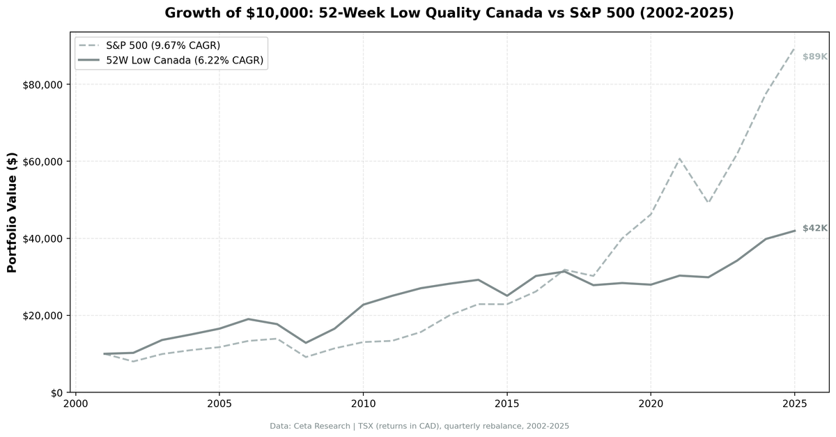
The terminal wealth gap is large. $10k grew to $41,932 here vs $89,485 in SPY. The CAGR difference of 3.45 percentage points compounds into a 2:1 wealth ratio over 24 years.
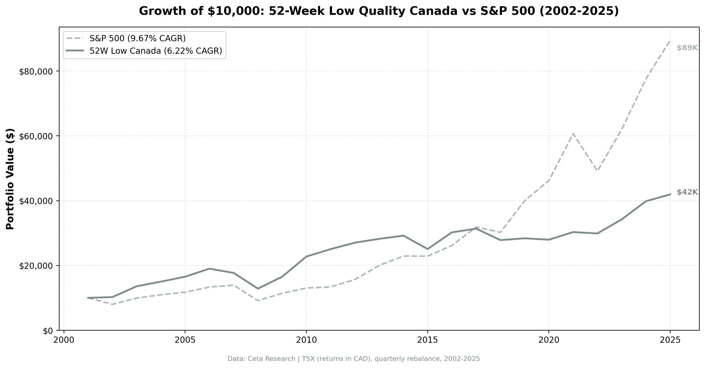
$10k invested in January 2002. Canada portfolio (blue) reaches $41,932 vs SPY (grey) $89,485 by December 2025.
Year-by-Year
| Year | Portfolio | S&P 500 | Excess |
|---|---|---|---|
| 2002 | +2.45% | -19.92% | +22.37% |
| 2003 | +32.62% | +24.12% | +8.50% |
| 2004 | +18.33% | +10.25% | +8.08% |
| 2005 | +14.67% | +7.21% | +7.46% |
| 2006 | +22.84% | +13.65% | +9.19% |
| 2007 | +12.41% | +4.40% | +8.01% |
| 2008 | -27.44% | -34.31% | +6.87% |
| 2009 | +28.67% | +24.73% | +3.94% |
| 2010 | +37.69% | +14.31% | +23.38% |
| 2011 | +10.06% | +2.46% | +7.60% |
| 2012 | +8.93% | +17.09% | -8.16% |
| 2013 | +4.33% | +27.77% | -23.44% |
| 2014 | +4.98% | +14.50% | -9.52% |
| 2015 | -12.87% | -0.07% | -12.80% |
| 2016 | +20.49% | +14.45% | +6.04% |
| 2017 | +9.14% | +21.64% | -12.50% |
| 2018 | -8.76% | -5.23% | -3.53% |
| 2019 | +6.44% | +32.31% | -25.87% |
| 2020 | -3.21% | +15.64% | -18.85% |
| 2021 | +19.87% | +31.33% | -11.46% |
| 2022 | -1.42% | -18.99% | +17.57% |
| 2023 | +14.50% | +26.00% | -11.50% |
| 2024 | +11.23% | +25.28% | -14.05% |
The 2002 to 2011 decade is where this strategy earns its keep. The TSX's resource-heavy composition provided natural protection during the dot-com bust, and the strategy outperformed SPY for nine of the first ten years. Energy and mining stocks at 52-week lows with strong balance sheets recovered when commodity prices normalized.
The 2012 to 2015 stretch is the rough patch. Three consecutive years of large underperformance: -8.16%, -23.44%, -9.52%. US equity markets ran hard on technology and growth names while Canadian resource companies stagnated. The strategy's compressed-P/E contrarian bets simply sat there.
2015 stands out. Oil prices fell from $60 to $30. TSX energy companies with Piotroski scores of 7 or higher at the start of 2015 kept falling as oil collapsed. The quality filter doesn't protect against commodity cycle deterioration when commodity prices move faster than annual financial statements can capture.
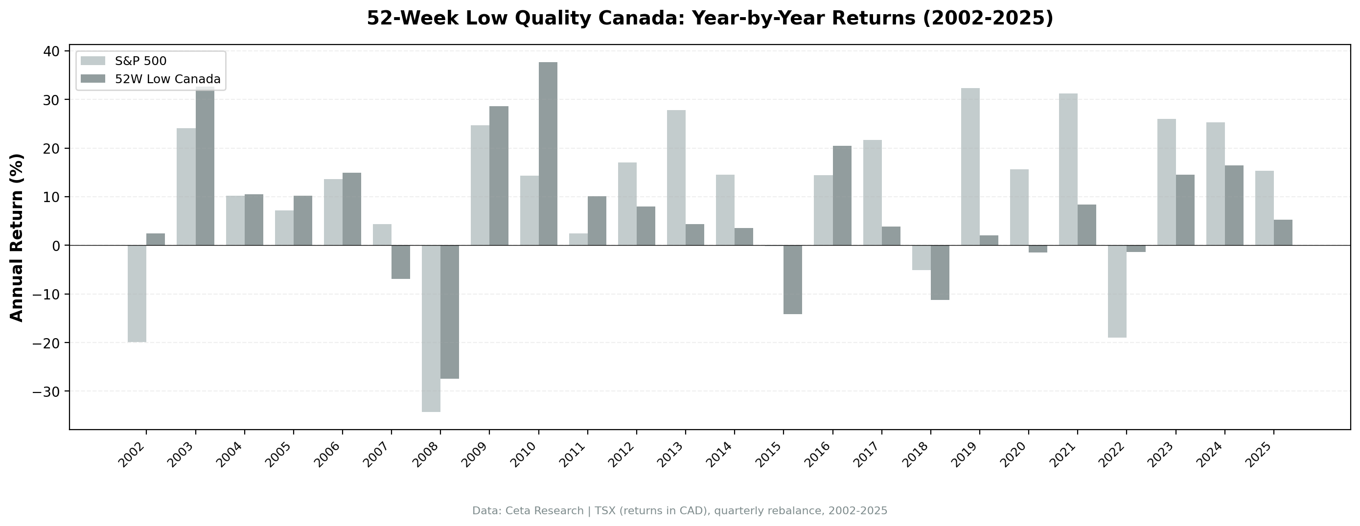
Year-by-year comparison. The early decade outperformance (2002–2011) gives way to persistent underperformance during US-led growth periods.
Why the TSX Behaves This Way
The TSX has a structurally different sector composition from the S&P 500. As of 2025, roughly 35% of the TSX is financials, 20% is energy, and 15% is materials. Technology is under 10%. Compare that to the S&P 500 where technology and tech-adjacent companies represent over 30% of index weight.
This composition has two effects on a 52-week low quality screen.
First, the signal fires more reliably. Energy and mining companies trade on commodity cycles. When oil falls from $80 to $50, quality producers hit 52-week lows. Those lows are a function of commodity price, not business quality. When oil recovers, the stocks recover. A Piotroski filter is very good at identifying which energy companies have the financial strength to wait out the cycle.
Second, the strategy misses US technology-driven rallies entirely. In 2019 and 2023, the S&P 500 surged on FAANG and AI names. No TSX-listed stock participates in that. A Canadian 52-week low screen with quality filters will hold a portfolio of banks, pipelines, and miners. Those businesses have nothing to do with US semiconductor demand or cloud software valuations.
The down-capture of 71.72% is higher than India's 42.88%. Canada doesn't protect as well during crashes, but it also doesn't have India's volatility. When SPY falls, Canadian quality stocks fall roughly 72% as much. That's not exceptional protection, but it's real. The max drawdown of -36.61% vs SPY's -45.53% is the cleanest summary of the defensive characteristic.
A Canadian investor benchmarking against the TSX Composite (which has historically returned 5-7% annually) would see 6.22% as roughly matching the index. The comparison to SPY at 9.67% looks unfavorable, but that's partly a currency effect and partly the different composition of the two indexes.
Part of a Series: Global | US | Switzerland | India | Hong Kong | Germany | China
Run It Yourself
-- 52-Week Low Quality Screen: TSX (Canada)
-- Stocks within 15% of 52-week low with Piotroski F-Score >= 7
-- Point-in-time with 45-day filing lag
WITH price_history AS (
 SELECT
 e.symbol,
 e.date,
 e.adjClose,
 MIN(e.adjClose) OVER (
 PARTITION BY e.symbol
 ORDER BY e.date
 ROWS BETWEEN 251 PRECEDING AND CURRENT ROW
 ) AS low_52wk
 FROM read_parquet('/opt/insydia/data/data_source=fmp/tick_data/eod/*.parquet') e
 JOIN read_parquet('/opt/insydia/data/data_source=fmp/company/profile/*.parquet') p
 ON e.symbol = p.symbol
 WHERE p.exchange = 'TSX'
 AND e.date <= CURRENT_DATE
 AND e.date >= CURRENT_DATE - INTERVAL '400' DAY
),
latest_price AS (
 SELECT symbol, adjClose AS current_price, low_52wk,
 ROW_NUMBER() OVER (PARTITION BY symbol ORDER BY date DESC) AS rn
 FROM price_history
 WHERE date <= CURRENT_DATE
),
near_low AS (
 SELECT symbol, current_price, low_52wk,
 (current_price / low_52wk - 1) AS pct_above_low
 FROM latest_price
 WHERE rn = 1 AND low_52wk > 0
 AND (current_price / low_52wk - 1) < 0.15
),
piotroski AS (
 SELECT
 i.symbol,
 i.date,
 CASE WHEN i.netIncome > 0 THEN 1 ELSE 0 END AS f1_net_income,
 CASE WHEN c.operatingCashFlow > 0 THEN 1 ELSE 0 END AS f2_ocf,
 CASE WHEN (i.netIncome / NULLIF(b.totalAssets, 0)) >
 LAG(i.netIncome / NULLIF(b.totalAssets, 0)) OVER (PARTITION BY i.symbol ORDER BY i.date)
 THEN 1 ELSE 0 END AS f3_roa_improving,
 CASE WHEN c.operatingCashFlow > i.netIncome THEN 1 ELSE 0 END AS f4_accruals,
 CASE WHEN (b.longTermDebt / NULLIF(b.totalAssets, 0)) <
 LAG(b.longTermDebt / NULLIF(b.totalAssets, 0)) OVER (PARTITION BY b.symbol ORDER BY b.date)
 THEN 1 ELSE 0 END AS f5_leverage,
 CASE WHEN (b.totalCurrentAssets / NULLIF(b.totalCurrentLiabilities, 0)) >
 LAG(b.totalCurrentAssets / NULLIF(b.totalCurrentLiabilities, 0)) OVER (PARTITION BY b.symbol ORDER BY b.date)
 THEN 1 ELSE 0 END AS f6_liquidity,
 CASE WHEN i.weightedAverageShsOut <=
 LAG(i.weightedAverageShsOut) OVER (PARTITION BY i.symbol ORDER BY i.date)
 THEN 1 ELSE 0 END AS f7_no_dilution,
 CASE WHEN (i.grossProfit / NULLIF(i.revenue, 0)) >
 LAG(i.grossProfit / NULLIF(i.revenue, 0)) OVER (PARTITION BY i.symbol ORDER BY i.date)
 THEN 1 ELSE 0 END AS f8_gross_margin,
 CASE WHEN (i.revenue / NULLIF(b.totalAssets, 0)) >
 LAG(i.revenue / NULLIF(b.totalAssets, 0)) OVER (PARTITION BY i.symbol ORDER BY i.date)
 THEN 1 ELSE 0 END AS f9_asset_turnover
 FROM read_parquet('/opt/insydia/data/data_source=fmp/statements/income_statement/*.parquet') i
 JOIN read_parquet('/opt/insydia/data/data_source=fmp/statements/balance_sheet_statement/*.parquet') b
 ON i.symbol = b.symbol AND i.date = b.date AND i.period = b.period
 JOIN read_parquet('/opt/insydia/data/data_source=fmp/statements/cash_flow_statement/*.parquet') c
 ON i.symbol = c.symbol AND i.date = c.date AND i.period = c.period
 WHERE i.period = 'FY'
 AND CAST(i.date AS DATE) <= CURRENT_DATE - INTERVAL '45' DAY
),
piotroski_scored AS (
 SELECT symbol,
 (f1_net_income + f2_ocf + f3_roa_improving + f4_accruals +
 f5_leverage + f6_liquidity + f7_no_dilution + f8_gross_margin + f9_asset_turnover) AS fscore,
 ROW_NUMBER() OVER (PARTITION BY symbol ORDER BY date DESC) AS rn
 FROM piotroski
),
quality AS (
 SELECT k.symbol, k.marketCap,
 ROW_NUMBER() OVER (PARTITION BY k.symbol ORDER BY k.date DESC) AS rn
 FROM read_parquet('/opt/insydia/data/data_source=fmp/statements/key_metrics/*.parquet') k
 WHERE CAST(k.date AS DATE) <= CURRENT_DATE - INTERVAL '45' DAY
 AND k.period = 'FY'
)
SELECT
 n.symbol,
 ROUND(n.current_price, 2) AS current_price,
 ROUND(n.low_52wk, 2) AS low_52wk,
 ROUND(n.pct_above_low * 100, 2) AS pct_above_low,
 ps.fscore AS piotroski_score,
 ROUND(q.marketCap / 1e6, 0) AS mktcap_mm
FROM near_low n
JOIN piotroski_scored ps ON n.symbol = ps.symbol AND ps.rn = 1
JOIN quality q ON n.symbol = q.symbol AND q.rn = 1
WHERE ps.fscore >= 7
 AND q.marketCap > 100000000
ORDER BY n.pct_above_low ASC
LIMIT 30
Run this screen on Ceta Research →
Limitations
Currency mismatch. Returns are in CAD. The benchmark is in USD. CAD/USD fluctuations affect the comparison independently of the strategy's actual performance. Over the 2002–2025 period, CAD depreciation vs USD weighs against the Canadian portfolio when measured against SPY.
Energy concentration risk. The TSX's heavy energy weighting means this screen regularly concentrates in oil and gas companies when commodity prices correct. In 2015, that created correlated losses when oil fell from $60 to $30. Quality companies can still fall 40% if the commodity they depend on collapses.
The 2013–2014–2015 gap. Three consecutive years of significant underperformance totaling roughly -45 percentage points of cumulative excess return. A real investor would need conviction to hold through that stretch.
Win rate of 43.16%. Fewer than half of the 95 quarters beat SPY. The strategy wins when it wins big (2002, 2010, 2022) but loses modestly in many of the remaining quarters. The skew is positive but the frequency of beating the benchmark is low.
Annual statement lag. With quarterly rebalancing and a 45-day filing lag, the Piotroski score reflects annual statements. A company whose energy revenues collapse mid-year won't trigger a portfolio exit until the next rebalance after the annual filing. The 2015 oil crash demonstrated this timing gap clearly.
Run It Yourself
Explore the data behind this analysis on Ceta Research. Query our financial data warehouse with SQL, build custom screens, and run your own backtests across 70,000+ stocks on 20 exchanges.
Data: Ceta Research (FMP financial data warehouse), 2002–2025. Full methodology: backtests/METHODOLOGY.md. Backtest code: backtests/52-week-low/. Past performance doesn't guarantee future results. Educational content only, not investment advice.