Sector P/E Compression: Buying Cheap Industries Based on Valuation

Sector P/E Compression: Buying Cheap Industries Based on Valuation Mean Reversion
Everyone talks about buying cheap stocks. What about buying cheap sectors?
Contents
- The Strategy
- Backtest Results (2005-2025, With Costs)
- How We Calculate Sector P/E
- The Z-Score Signal
- When Sector Compression Works
- When Sector Compression Struggles
- The Screen
- The Academic Foundation
- Practical Considerations
- Limitations
- References
When an entire industry trades at a P/E ratio more than one standard deviation below its 5-year average, something interesting is happening. Either the market has correctly priced in permanent decline, or you're looking at a mean reversion opportunity.
Campbell and Shiller (1988) showed that aggregate valuations mean-revert over time. The same pattern holds at the sector level.
The Strategy
Sector P/E compression is a value-based approach to sector allocation.
Instead of buying the cheapest stocks, buy the cheapest sectors. Instead of comparing a stock to the market, compare a sector to itself.
The signal: when a sector's aggregate P/E ratio falls more than 1 standard deviation below its 5-year average, it's compressed. History suggests compressed sectors tend to revert toward their mean over 2-5 years.
Why it works: Sectors don't compress randomly. They compress due to cyclical factors (Energy in downturns), regulatory fears (Financials after crises), or sentiment swings (Tech after bubbles). These factors tend to reverse.
Why it's hard: Mean reversion takes time. You need patience and conviction to hold a hated sector while waiting for sentiment to turn.
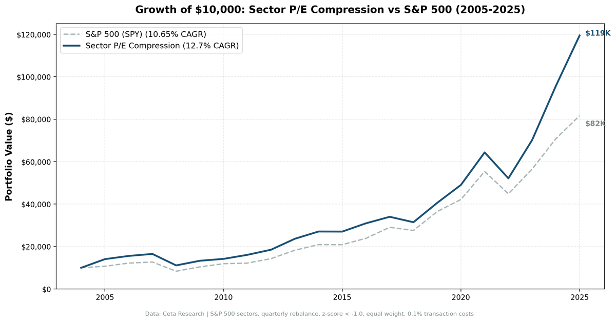
Backtest Results (2005-2025, With Costs)
| Strategy | CAGR | Final Value ($10k) | Sharpe | Max Drawdown | Volatility |
|---|---|---|---|---|---|
| Sector P/E Compression | 12.70% | $119,431 | 0.647 | 45.57% | 16.54% |
| SPY (Buy & Hold) | 10.65% | $81,668 | 0.520 | 45.53% | 16.64% |
The strategy outperformed SPY by 2.05% annually over 21 years. On $10,000 invested, that's $37,763 more at the end.
The down-capture ratio of 67.6% stands out. When SPY had a losing quarter, this strategy lost on average only 67.6% as much. You get most of the upside (95.6% up-capture) with meaningfully less downside exposure in normal bear quarters.
Both strategies hit similar max drawdowns (45.57% vs 45.53%) because the 2008 crash hit everything hard. But quarter-by-quarter, the compression tilt provides a real buffer during selloffs.
How We Calculate Sector P/E
Sector P/E isn't a simple average of constituent P/Es. That would give equal weight to a $10B company and a $500B company.
We use market-cap weighted aggregate P/E:
Sector P/E = Sum(Market Cap) / Sum(Earnings)
This is equivalent to:
Sector P/E = Sum(Market Cap) / Sum(Market Cap / PE)
A sector with $5 trillion market cap and $250 billion in earnings has a P/E of 20x. This captures the economic reality better than averaging individual P/Es.
The Z-Score Signal
Knowing a sector's current P/E is step one. Step two: comparing it to history.
We calculate a z-score:
Z-Score = (Current PE - 5-Year Average PE) / Standard Deviation
A z-score of -1.5 means the sector is trading 1.5 standard deviations below its historical average. That's compressed.
| Z-Score | Interpretation |
|---|---|
| < -1.0 | COMPRESSED - Consider overweight |
| -1.0 to 1.0 | NORMAL - Market weight |
| > 1.0 | STRETCHED - Consider underweight |
When Sector Compression Works
Early cycle rotations
In 2005, beaten-down post-dot-com sectors reversed hard. The strategy returned +40.65% while SPY gained 7.17%, a 33.47% excess in a single year. Valuation compression built up over 2001-2004 unwound all at once.
Post-crisis recoveries
In 2011, compressed Financials and Energy sectors drove a 13.35% return vs SPY's 2.46% (+10.89% excess). The strategy is consistently positioned in sectors that lagged during crises, which creates outsized recovery potential.
Sustained sector rotations
The most recent three-year run shows the signal working across a full market cycle:
| Year | Strategy | SPY | Excess |
|---|---|---|---|
| 2023 | +34.59% | +26.00% | +8.59% |
| 2024 | +36.33% | +25.28% | +11.05% |
| 2025 | +24.85% | +15.34% | +9.51% |
Combined excess over three years: roughly +29% cumulative alpha during a period when the market itself was strong.
When Sector Compression Struggles
Sustained growth market dominance
When Technology persistently commands premium valuations and nothing compresses, the strategy often reverts to SPY or underperforms. In 2017, Tech's dominance meant compressed sectors lagged the index badly (-11.74% excess). The strategy isn't wrong, it's waiting.
The 2022 case: when P/E breaks down for cyclicals
The strategy missed the 2022 Energy rally entirely. Our backtest shows 0.0% excess that year, the portfolio held SPY and matched the index exactly (-18.99%).
What happened: COVID wiped out FY2020 earnings for most Energy S&P 500 members. When we filter for positive P/E ratios, only 10 of 23 Energy stocks qualified. Those 10 profitable survivors showed high P/Es (~47x average), making Energy appear stretched not compressed in the z-score calculation. The signal didn't fire.
This is the core limitation of P/E compression for cyclical sectors. When earnings temporarily collapse, P/E-based signals can invert. A better approach for Energy and Basic Materials during commodity troughs is P/B or EV/EBITDA. The strategy as implemented is most reliable for non-cyclical compression scenarios.
Short horizons
Mean reversion at the sector level takes 2-5 years. If you need results in 6 months, this isn't your strategy.
The Screen
Run this on live data to see which sectors are currently compressed:
WITH sector_members AS (
 SELECT DISTINCT symbol, sector
 FROM sp500_constituent
 WHERE sector IS NOT NULL AND sector != ''
),
latest_pe AS (
 SELECT r.symbol, r.priceToEarningsRatio AS pe,
 r.dateEpoch AS filing_epoch,
 ROW_NUMBER() OVER (PARTITION BY r.symbol ORDER BY r.dateEpoch DESC) AS rn
 FROM financial_ratios r
 JOIN sector_members s ON r.symbol = s.symbol
 WHERE r.period = 'FY'
 AND r.priceToEarningsRatio > 0
 AND r.priceToEarningsRatio < 200
),
latest_mcap AS (
 SELECT m.symbol, m.marketCap,
 ROW_NUMBER() OVER (PARTITION BY m.symbol ORDER BY m.dateEpoch DESC) AS rn
 FROM key_metrics m
 JOIN sector_members s ON m.symbol = s.symbol
 WHERE m.period = 'FY' AND m.marketCap > 0
),
current_sector_pe AS (
 SELECT sm.sector,
 COUNT(*) AS n_stocks,
 SUM(lm.marketCap) / NULLIF(SUM(lm.marketCap / lp.pe), 0) AS current_pe
 FROM sector_members sm
 JOIN latest_pe lp ON sm.symbol = lp.symbol AND lp.rn = 1
 JOIN latest_mcap lm ON sm.symbol = lm.symbol AND lm.rn = 1
 WHERE lp.pe > 0 AND lm.marketCap > 0
 GROUP BY sm.sector HAVING COUNT(*) >= 3
),
historical_annual AS (
 SELECT sm.sector,
 EXTRACT(YEAR FROM CAST(r.date AS DATE)) AS yr,
 SUM(m.marketCap) / NULLIF(SUM(m.marketCap / r.priceToEarningsRatio), 0) AS sector_pe
 FROM financial_ratios r
 JOIN sector_members sm ON r.symbol = sm.symbol
 JOIN key_metrics m ON r.symbol = m.symbol
 AND ABS(CAST(r.dateEpoch AS BIGINT) - CAST(m.dateEpoch AS BIGINT)) < 86400 * 60
 WHERE r.period = 'FY'
 AND r.priceToEarningsRatio > 0 AND r.priceToEarningsRatio < 200
 AND m.marketCap > 0
 AND EXTRACT(YEAR FROM CAST(r.date AS DATE)) >= EXTRACT(YEAR FROM CURRENT_DATE) - 5
 GROUP BY sm.sector, yr HAVING COUNT(DISTINCT r.symbol) >= 3
),
sector_stats AS (
 SELECT sector, AVG(sector_pe) AS avg_pe_5yr, STDDEV(sector_pe) AS std_pe_5yr, COUNT(*) AS n_years
 FROM historical_annual GROUP BY sector HAVING COUNT(*) >= 3
)
SELECT
 c.sector,
 c.n_stocks,
 ROUND(c.current_pe, 1) AS current_pe,
 ROUND(s.avg_pe_5yr, 1) AS avg_pe_5yr,
 ROUND((c.current_pe - s.avg_pe_5yr) / NULLIF(s.std_pe_5yr, 0), 2) AS z_score,
 CASE
 WHEN (c.current_pe - s.avg_pe_5yr) / NULLIF(s.std_pe_5yr, 0) < -1.0 THEN 'COMPRESSED'
 WHEN (c.current_pe - s.avg_pe_5yr) / NULLIF(s.std_pe_5yr, 0) > 1.0 THEN 'STRETCHED'
 ELSE 'NORMAL'
 END AS signal
FROM current_sector_pe c
JOIN sector_stats s ON c.sector = s.sector
ORDER BY z_score ASC;
The Academic Foundation
Campbell & Shiller (1988): Established that aggregate stock prices, earnings, and dividends are cointegrated and mean-reverting. Valuation ratios predict long-term returns.
Lakonishok, Shleifer & Vishny (1994): Showed that value strategies (buying low P/E, low P/B) outperform because investors extrapolate past performance too far into the future. Compressed valuations revert.
Fama & French (1992): Documented the value factor (HML). Cheap stocks outperform expensive stocks on average. This extends to sectors.
The academic consensus: valuation compression predicts higher future returns over multi-year horizons. The challenge is implementation patience.
Practical Considerations
Use sector ETFs. XLK, XLE, XLF, XLV, XLY, XLP, XLI, XLB, XLU, XLRE, XLC. Low cost, liquid, no single-stock risk.
Quarterly rebalancing. Check z-scores at quarter end. Don't chase intra-quarter noise.
The cyclical limitation. P/E compression works best for non-cyclical sectors. For Energy, Basic Materials, and other earnings-volatile sectors, a temporary earnings collapse can make an actually-cheap sector appear expensive. Consider supplementing with P/B or EV/EBITDA for these sectors.
When no sectors are compressed, hold SPY. Roughly 38% of quarters in our backtest had no compressed sectors. The strategy defaults to SPY rather than forcing positions.
Patience required. A compressed sector might stay compressed for 6-12 months before reverting.
Limitations
Survivorship bias. This backtest uses the current S&P 500 constituent list for all historical sector mapping. Companies removed from the index before 2026 are excluded from historical P/E calculations. Impact is modest because the signal is sector-level, not individual stock selection, but it's real.
P/E signal breaks for cyclicals. During earnings troughs in Energy and Basic Materials, the positive-P/E filter creates survivorship distortion within the sector. The visible subset shows inflated P/Es, making the sector look expensive when it may actually be cheap. The 2022 Energy miss is a direct result of this.
FY data lag. We apply a 45-day lag after fiscal year-end before using P/E data. This prevents look-ahead bias but means signals are based on annual data that may be 12-18 months old.
References
- Campbell, J. Y., & Shiller, R. J. (1988). Stock prices, earnings, and expected dividends. The Journal of Finance, 43(3), 661-676.
- Lakonishok, J., Shleifer, A., & Vishny, R. W. (1994). Contrarian investment, extrapolation, and risk. The Journal of Finance, 49(5), 1541-1578.
- Fama, E. F., & French, K. R. (1992). The cross-section of expected stock returns. The Journal of Finance, 47(2), 427-465.
Run It Yourself
Explore the data behind this analysis on Ceta Research. Query our financial data warehouse with SQL, build custom screens, and run your own backtests across 70,000+ stocks on 20 exchanges.
Data: Ceta Research, S&P 500 constituents (sp500_constituent, financial_ratios, key_metrics, stock_eod tables) Backtest: 2005-2025, quarterly rebalance, z-score < -1.0 signal, 0.1% transaction costs Past performance doesn't guarantee future results. This is educational content, not investment advice.