Sector Correlation Regimes: Why the Signal Works But the Trade Doesn't
We built a regime-detection system using 60-day rolling sector correlations and tested it on 26 years of US market data. The strategy correctly identified every major stress period. It still underperformed SPY by 1.89% annually.

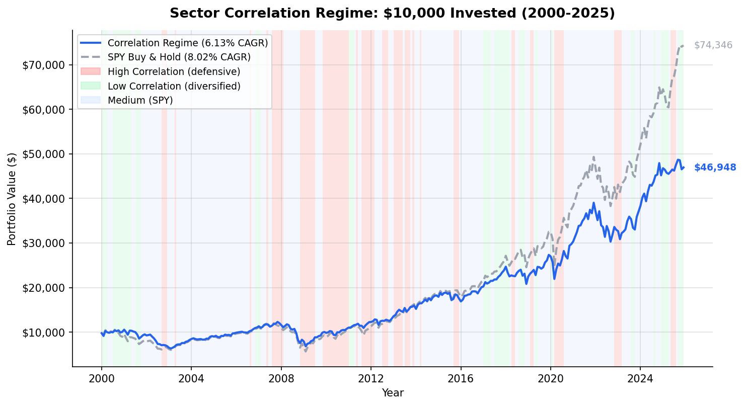
When all sectors move together, diversification fails. The idea: detect those moments early and rotate into defensive positions before the damage compounds. We built exactly that system and tested it on 25 years of US market data. The result is a clean lesson in the difference between a useful risk indicator and an actionable trading signal.
Contents
- The Setup
- Results
- Where the Time Was Spent
- Year-by-Year
- Why It Underperforms
- When Correlations Actually Spiked
- What Correlation Monitoring Is Actually For
- Current Reading
- The Finding
- Academic Basis
The Setup
Universe: 9 S&P 500 Sector SPDR ETFs (XLK, XLE, XLF, XLV, XLY, XLP, XLI, XLB, XLU) Signal: 60-day rolling average pairwise correlation across all 36 sector pairs Rebalance: Monthly Period: January 2000 to December 2025 (26 years, 312 months) Transaction costs: 0.1% per side on regime changes
The signal is a single number: the average Pearson correlation across every possible pair of the 9 sector ETFs. That's 36 pairs, averaged monthly.
| Regime | Condition | Allocation |
|---|---|---|
| High | avg corr > 0.70 | Defensive sectors: XLU + XLV + XLP (equal weight) |
| Medium | 0.40 to 0.70 | SPY (buy and hold) |
| Low | avg corr < 0.40 | All 9 sector ETFs (equal weight) |
The hypothesis: when correlations spike, everything falls together. Rotating to utilities, healthcare, and consumer staples before the collapse should limit damage. When correlations are low, diversification works and spreading across all sectors captures the premium.
Results
| Metric | Correlation Regime | SPY Buy & Hold |
|---|---|---|
| CAGR | 6.13% | 8.02% |
| Total Return (26yr) | 369% | 643% |
| Final Value ($10k) | $46,948 | $74,346 |
| Max Drawdown | -44.5% | -52.9% |
| Sharpe Ratio | 0.292 | 0.366 |
| Annualized Volatility | 14.1% | 16.4% |
The strategy underperformed SPY by 1.89% annually. Over 26 years, that gap compounded into $27,000 less wealth on a $10,000 investment.
The drawdown protection is real: -44.5% vs -52.9%. Volatility is lower: 14.1% vs 16.4%. But none of that closes the return gap. The strategy takes on 87% of SPY's risk while delivering 77% of SPY's return. That's a bad tradeoff.
Where the Time Was Spent
| Regime | Months | % of Time | Avg Annual Return |
|---|---|---|---|
| High (> 0.70) | 74 | 23.7% | +12.3% |
| Medium (0.40-0.70) | 188 | 60.3% | +7.4% |
| Low (< 0.40) | 50 | 16.0% | -0.6% |
The high-correlation regime returned +12.3% annually. The defensive positioning worked when it engaged. But the strategy was in that regime only 24% of the time.
The real problem is the low-correlation regime. Equal-weighting all 9 sectors returned -0.6% annually in those periods. SPY is increasingly dominated by technology: in 2024, the top 10 holdings were ~35% of index weight. Equal-weighting gives tech 1/9 of the portfolio. During low-correlation periods, sector dispersion actually helps SPY's concentrated positions, not the equal-weight spread.
Year-by-Year
| Year | Strategy | SPY | Excess |
|---|---|---|---|
| 2000 | +0.5% | -10.5% | +11.0% |
| 2001 | -5.6% | -9.2% | +3.6% |
| 2002 | -27.8% | -19.9% | -7.9% |
| 2007 | +8.8% | +4.4% | +4.4% |
| 2008 | -30.9% | -34.3% | +3.4% |
| 2010 | +7.1% | +14.3% | -7.2% |
| 2011 | +13.9% | +2.5% | +11.5% |
| 2018 | -12.7% | -5.2% | -7.5% |
| 2022 | -15.5% | -19.0% | +3.5% |
| 2023 | +12.4% | +26.0% | -13.6% |
| 2024 | +21.9% | +25.3% | -3.4% |
| 2025 | +3.9% | +17.9% | -14.0% |
The strategy protected during dot-com (2000-2001) and the 2011 European debt crisis. It fell short during the 2008 financial crisis: -30.9% vs -34.3%. The defensive shift came after the initial drop, not before it.
The recent years are rough. 2023 (-13.6% excess), 2025 (-14.0% excess). The current low-correlation regime means equal-weighting sectors while SPY's tech concentration keeps compounding.
Why It Underperforms
The timing problem. Correlation spikes after markets start falling. The 60-day rolling window looks backward. By the time average correlation crosses 0.70, the index has often already dropped 15-20%. Defensive positioning captures some of the remaining downside protection but misses the optimal entry.
The low-correlation trap. The strategy is most active (non-SPY) during two regime types. High correlation: defensive tilt works. Low correlation: equal-weight sectors underperform a tech-heavy index. The regime the strategy is supposed to benefit from is actually its worst performer.
65 regime changes over 26 years. That's 2.5 switches per year on average. Each change incurs 0.1% transaction cost. More importantly, each switch risks being wrong about regime persistence. The strategy paid costs to enter low-correlation periods that returned -0.6% annually.
The medium regime captured the bulk of SPY's returns. 60% of the time, the strategy held SPY directly. During those periods, SPY returned +7.4% annually. Structural SPY underperformance in those months accumulated over 188 periods.
When Correlations Actually Spiked
These are the confirmed high-correlation periods (avg > 0.70):
| Period | Notes |
|---|---|
| 2008-2010 | Financial crisis + recovery + European debt fears |
| 2011-2013 | European sovereign debt crisis + QE rounds |
| 2015-2016 | China slowdown + commodity crash |
| 2022-2023 | Fed rate hiking cycle |
The strategy correctly identified each of these stress periods. But timing the entry and exit consistently is hard. Correlations don't snap to 0.71 and hold there. They fluctuate around thresholds, generating false switches.
What Correlation Monitoring Is Actually For
This backtest doesn't invalidate correlation monitoring as a risk tool. It shows the limits of using it as a binary trading trigger.
Better applications:
Position sizing. When average sector correlation rises above 0.6, your equity positions become correlated. The diversification you're counting on isn't there. Reduce gross exposure rather than rotating sectors.
Hedge effectiveness. Correlations tell you whether your sector hedges are working. If XLK and XLF are both trading at 0.9 correlation to SPY, a sector hedge in one doesn't protect against the other.
Regime context. High correlation doesn't mean sell. It means know what you own. Your "diversified" 9-sector portfolio is behaving like a single bet on market direction.
Risk management overlay. For a portfolio already holding individual stocks, correlation spikes are a signal to check concentration, not to time rotations.
Current Reading
As of March 2026, the current regime is LOW (avg correlation: 0.243).
That means sector returns are diverging. Energy (+6.8% over 30 days), Utilities (+8.9%), while Financials (-6.6%) and Consumer Discretionary (-4.5%) have moved in the opposite direction. Diversification is working at the sector level right now.
According to the strategy, the correct allocation is equal weight across all 9 sector ETFs. The backtest says that has historically been the weakest regime for this approach.
Check the current reading yourself:
WITH daily_returns AS (
    SELECT
        symbol,
        CAST(date AS DATE) as trade_date,
        (adjClose - LAG(adjClose) OVER (PARTITION BY symbol ORDER BY date))
            / LAG(adjClose) OVER (PARTITION BY symbol ORDER BY date) AS daily_return
    FROM stock_eod
    WHERE symbol IN ('XLK', 'XLE', 'XLF', 'XLV', 'XLY', 'XLP', 'XLI', 'XLB', 'XLU')
      AND CAST(date AS DATE) >= CURRENT_DATE - INTERVAL '90 days'
),
pivot_returns AS (
    SELECT
        trade_date,
        MAX(CASE WHEN symbol = 'XLK' THEN daily_return END) as xlk,
        MAX(CASE WHEN symbol = 'XLE' THEN daily_return END) as xle,
        MAX(CASE WHEN symbol = 'XLF' THEN daily_return END) as xlf,
        MAX(CASE WHEN symbol = 'XLV' THEN daily_return END) as xlv,
        MAX(CASE WHEN symbol = 'XLY' THEN daily_return END) as xly,
        MAX(CASE WHEN symbol = 'XLP' THEN daily_return END) as xlp,
        MAX(CASE WHEN symbol = 'XLI' THEN daily_return END) as xli,
        MAX(CASE WHEN symbol = 'XLB' THEN daily_return END) as xlb,
        MAX(CASE WHEN symbol = 'XLU' THEN daily_return END) as xlu
    FROM daily_returns
    GROUP BY trade_date
)
SELECT
    ROUND(CAST((
        CORR(xlk,xle)+CORR(xlk,xlf)+CORR(xlk,xlv)+CORR(xlk,xly)+CORR(xlk,xlp)+
        CORR(xlk,xli)+CORR(xlk,xlb)+CORR(xlk,xlu)+CORR(xle,xlf)+CORR(xle,xlv)+
        CORR(xle,xly)+CORR(xle,xlp)+CORR(xle,xli)+CORR(xle,xlb)+CORR(xle,xlu)+
        CORR(xlf,xlv)+CORR(xlf,xly)+CORR(xlf,xlp)+CORR(xlf,xli)+CORR(xlf,xlb)+
        CORR(xlf,xlu)+CORR(xlv,xly)+CORR(xlv,xlp)+CORR(xlv,xli)+CORR(xlv,xlb)+
        CORR(xlv,xlu)+CORR(xly,xlp)+CORR(xly,xli)+CORR(xly,xlb)+CORR(xly,xlu)+
        CORR(xlp,xli)+CORR(xlp,xlb)+CORR(xlp,xlu)+CORR(xli,xlb)+CORR(xli,xlu)+
        CORR(xlb,xlu)
    ) / 36.0 AS DOUBLE), 3) as avg_pairwise_correlation
FROM pivot_returns
Run it: cetaresearch.com/data-explorer?q=4ZJtwqO5Hm
The Finding
Correlation as a risk indicator works. Correlation as a trading signal doesn't.
The strategy correctly identified every major stress period over 26 years. High-correlation regimes during 2008-2010, 2011-2013, and 2022-2023 were real. The defensive rotation in those periods returned +12.3% annually.
But the signal lags the crisis. By the time 60-day correlations cross 0.70, markets have usually already moved. And the low-correlation regime, which sounds like the good scenario for diversification, actually hurt the strategy because SPY's index concentration outperforms equal-weight sector exposure.
The lesson isn't to ignore correlations. It's that regime-detection strategies need the regime to persist long enough after detection to justify the cost of repositioning. With sector correlations, the lag between signal and reality makes that nearly impossible to do profitably.
Academic Basis
- Longin, F. & Solnik, B. (2001). "Extreme Correlation of International Equity Markets." Journal of Finance, 56(2), 649-676. Documents that correlations increase during bear markets.
- Kritzman, M. et al. (2012). "Regime Shifts: Implications for Dynamic Strategies." Financial Analysts Journal, 68(3), 22-39. Studies dynamic allocation across market regimes.
Data: FMP financial data via Ceta Research, S&P 500 sector ETFs (stock_eod), 2000-2025. Transaction costs included (0.1% per side on regime change). Past performance does not guarantee future results.