Pairs Trading Backtest: 20 Years of US Results

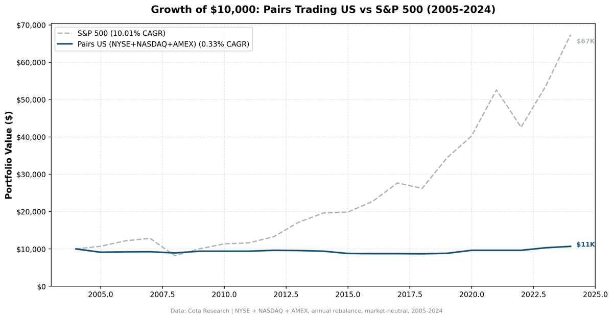
Twenty years, -0.50% CAGR, Sharpe of -0.81. That's the headline. The pairs trading strategy we covered in the first post in this series, correlation-based, same-sector, z-score entry, ran clean over 2005 through 2024 on US stocks. It didn't blow up. It also didn't make money. What it did do, in 2008 and a handful of other down years, was exactly what it's supposed to: stay flat while everything else fell apart.
Contents
- Method
- Year-by-Year Results
- The Six Cash Years
- When the Strategy Works
- Transaction Costs
- The Right Benchmark
- Current Pairs Screen
- Limitations
This post is the data. Year-by-year returns, six cash years explained, transaction cost drag, and the benchmark question that matters most for market-neutral strategies.
Method
Quick parameters for reference. The strategy is described in full in pairs-01.
| Parameter | Value |
|---|---|
| Universe | US stocks (NYSE, NASDAQ, AMEX) |
| Reconstitution | Annual |
| Pair selection | Same sector, correlation >= 0.70 (prior 12 months) |
| Hedge ratio | OLS (ordinary least squares) |
| Entry threshold | |z-score| > 1.5 |
| Position sizing | Equal-dollar, market-neutral |
| Execution | Next-day close (MOC) |
| Average active pairs | 5.4 (when invested) |
| Cash years | 6 out of 20 |
Year-by-Year Results
| Year | Portfolio | SPY | Excess | Active Pairs |
|---|---|---|---|---|
| 2005 | -8.79% | +7.17% | -15.97% | 7 |
| 2006 | -1.59% | +13.65% | -15.24% | 4 |
| 2007 | +0.46% | +4.40% | -3.94% | 4 |
| 2008 | -2.50% | -34.31% | +31.81% | 6 |
| 2009 | +1.59% | +24.73% | -23.14% | 5 |
| 2010 | 0.00% | +14.31% | -14.31% | 1 (cash) |
| 2011 | 0.00% | +2.46% | -2.46% | 1 (cash) |
| 2012 | +1.91% | +17.09% | -15.19% | 7 |
| 2013 | -1.56% | +27.77% | -29.33% | 7 |
| 2014 | -3.37% | +14.50% | -17.87% | 4 |
| 2015 | -4.72% | -0.12% | -4.60% | 5 |
| 2016 | -0.56% | +14.45% | -15.02% | 5 |
| 2017 | 0.00% | +21.64% | -21.64% | 1 (cash) |
| 2018 | -0.51% | -5.15% | +4.63% | 7 |
| 2019 | +1.21% | +32.31% | -31.10% | 4 |
| 2020 | 0.00% | +15.64% | -15.64% | 2 (cash) |
| 2021 | 0.00% | +31.26% | -31.26% | 0 (cash) |
| 2022 | 0.00% | -18.99% | +18.99% | 0 (cash) |
| 2023 | +6.73% | +26.00% | -19.28% | 4 |
| 2024 | +2.69% | +25.28% | -22.59% | 7 |
Win rate vs SPY: 3 out of 20 years (2008, 2018, 2022). Twenty years of data, three wins.
A few regimes stand out clearly. The post-GFC bull run from 2012 through 2016 was bad for the strategy: low volatility, high correlation across sectors, spread compression. Pairs that used to diverge and reconverge were moving together, so signals rarely fired, or fired and failed to converge. The 2005 loss of -8.79% was the worst absolute year, driven by seven active pairs that moved against the position and didn't recover within the holding window.
The recent stretch (2023, 2024) looks better in isolation. Two positive years in a row. But SPY returned 26% and 25% in those same years. The strategy captured single-digit returns while leaving 20 percentage points on the table annually.
The Six Cash Years
Cash years are years when the strategy held nothing, or too few pairs to trade. Zero return. They happened in 2010, 2011, 2017, 2020, 2021, and 2022.
2010 and 2011: The post-crisis recovery compressed cross-sector correlations in a way that broke the pair selection filter. In 2010, only one pair met the threshold, below the minimum-pairs rule (requiring at least three active positions). In 2011, same situation. SPY returned +14.3% and +2.5% in those years. The strategy earned nothing.
2017: A strong, low-volatility bull market. Same problem as 2010: correlations rose across the board, reducing inter-sector spread dispersion. Only one pair qualified. SPY returned +21.6%.
2020: COVID-driven volatility produced extreme divergences, but only two pairs met the entry threshold. Below the minimum-pairs rule. SPY returned +15.6%.
2021 and 2022: These two back-to-back cash years illustrate how the signal can fail in both bull and bear markets. In 2021, the meme stock era pushed idiosyncratic volatility through the roof. Pairs that historically correlated at 0.75+ were behaving randomly. No qualifying pairs formed. SPY returned +31.3%. In 2022, the opposite: rate-driven selloff hit every sector simultaneously. Cross-sector correlations spiked (everything fell together), and again no pairs met the threshold. SPY returned -19.0%. The strategy returned 0% in a year it should have helped most.
Cash years aren't just missed returns. They represent capital sitting idle with zero yield.
When the Strategy Works
The three years where pairs trading beat SPY are the only years you'd want the strategy in your portfolio.
2008: The clearest case. SPY dropped -34.3% as the financial system nearly collapsed. The pairs portfolio lost -2.5%. That's +31.8% excess return. The market-neutral construction, long one stock, short the correlated counterpart, meant equity beta exposure was near zero. Sector pairs that had historically co-moved continued to co-move even in the chaos, just at lower levels. The strategy held.
2018: A modest win. SPY fell -5.2% in a volatile year driven by trade war uncertainty and Fed rate hikes. The strategy lost -0.5%. Not profitable, but less bad. Seven active pairs that year.
2022: Cash. Not a "win" in any real sense. The strategy earned nothing but so did many investors (SPY -19%). Sitting in cash during a down year looks fine on paper. But the strategy didn't earn the T-bill rate during those months. It earned zero.
The pattern is consistent: the strategy offers crisis defense through genuine market-neutrality. Beta of 0.067 over 20 years is not luck. It's the structural result of holding long-short pairs. The problem is that crisis years are rare, the beta protection costs opportunity in bull markets, and even in the three "wins," the absolute return was negative or marginally positive.
Transaction Costs
Every pair trade involves four legs: buy stock A, short stock B on entry; close both on exit. Four commissions, four bid-ask spreads. At 5.4 average pairs, that's roughly 22 one-way transactions per year.
The -0.50% CAGR reported here is net of these costs. Before costs, the gross return is marginally higher, but not by much, because the strategy traded infrequently. Cash years had zero cost. Invested years averaged 5 pairs with one entry and one exit each.
The more important cost is implicit: six years of zero return with no T-bill compensation. A strategy sitting in cash earns nothing here. At 2% average short-term rates over the period, six cash years represent roughly 12% in foregone risk-free returns. That's a hidden drag that doesn't show up in transaction cost estimates but is real.
The Right Benchmark
The strategy's 10.28% SPY CAGR comparison exists in this post because readers will ask. But SPY is the wrong benchmark for a market-neutral strategy.
Market-neutral strategies target T-bill returns plus alpha. The appropriate benchmark is short-term rates: roughly 2% annualized over 2005-2024. Against that benchmark, a -0.50% CAGR strategy underperforms by about 2.5 percentage points per year. The strategy didn't just fail to generate alpha. It lost money.
Beta of 0.067 means the strategy absorbed almost none of the equity risk premium. That's the design. But it also means you don't get the equity return. If you run this in a portfolio as a diversifier, it reduces volatility and beta, but at a cost: you're adding negative expected return. For that trade-off to be worth making, you'd need the strategy to at least clear cash rates. It didn't.
Current Pairs Screen
The live pairs screen uses the same methodology: same-sector stocks, trailing 12-month correlation >= 0.70, current z-score computed via OLS hedge ratio.
WITH price_data AS (
  SELECT
    symbol,
    date,
    adjClose,
    AVG(adjClose) OVER (PARTITION BY symbol ORDER BY date ROWS BETWEEN 251 PRECEDING AND CURRENT ROW) AS ma252
  FROM stock_eod
  WHERE date >= CURRENT_DATE - INTERVAL '14 months'
),
returns AS (
  SELECT
    symbol,
    date,
    LN(adjClose / LAG(adjClose) OVER (PARTITION BY symbol ORDER BY date)) AS log_ret
  FROM price_data
),
sector_map AS (
  SELECT symbol, sector
  FROM profile
  WHERE exchange IN ('NYSE', 'NASDAQ', 'AMEX')
    AND marketCap > 500000000
    AND isActivelyTrading = TRUE
),
pairs AS (
  SELECT
    a.symbol AS sym_a,
    b.symbol AS sym_b,
    a.sector,
    CORR(ra.log_ret, rb.log_ret) AS correlation
  FROM sector_map a
  JOIN sector_map b ON a.sector = b.sector AND a.symbol < b.symbol
  JOIN returns ra ON a.symbol = ra.symbol
  JOIN returns rb ON b.symbol = rb.symbol AND ra.date = rb.date
  WHERE ra.date >= CURRENT_DATE - INTERVAL '12 months'
  GROUP BY a.symbol, b.symbol, a.sector
  HAVING CORR(ra.log_ret, rb.log_ret) >= 0.70
    AND COUNT(*) >= 200
)
SELECT
  sym_a,
  sym_b,
  sector,
  ROUND(correlation::numeric, 3) AS correlation
FROM pairs
ORDER BY correlation DESC
LIMIT 50
Live results: cetaresearch.com/data-explorer?q=z3_sysewqG
Limitations
A few things this backtest doesn't capture:
Short-selling constraints. Not every stock is shortable at all times. In crisis periods (exactly when the strategy should work), borrow rates spike and some stocks become unavailable. The backtest assumes frictionless shorts.
Minimum pairs rule. Years with fewer than three qualifying pairs are treated as cash. This protects against concentration but also creates the six zero-return years. A looser threshold (one or two pairs) would change the cash year count but add concentration risk.
Pair stability. Correlation is measured over trailing 12 months. Pairs that look correlated in the formation window often diverge in the trading window. This is the core risk in any statistical arbitrage strategy, and it's not fully captured by correlation alone.
Post-2015 regime. The US equity market has become increasingly factor-driven, with passive flows raising intra-sector correlations. That makes pair formation easier but convergence less reliable. The recent two-year positive run may reflect mean reversion in that dynamic, or it may not persist.
Data: FMP warehouse, 2005-2024. Returns are net of estimated transaction costs (4 one-way legs per pair). Next-day close execution (MOC). SPY used as equity benchmark for reference only. T-bills (~2% avg) are the appropriate benchmark for market-neutral strategies.