Pairs Trading Across 11 Global Exchanges: 20-Year Backtest Results

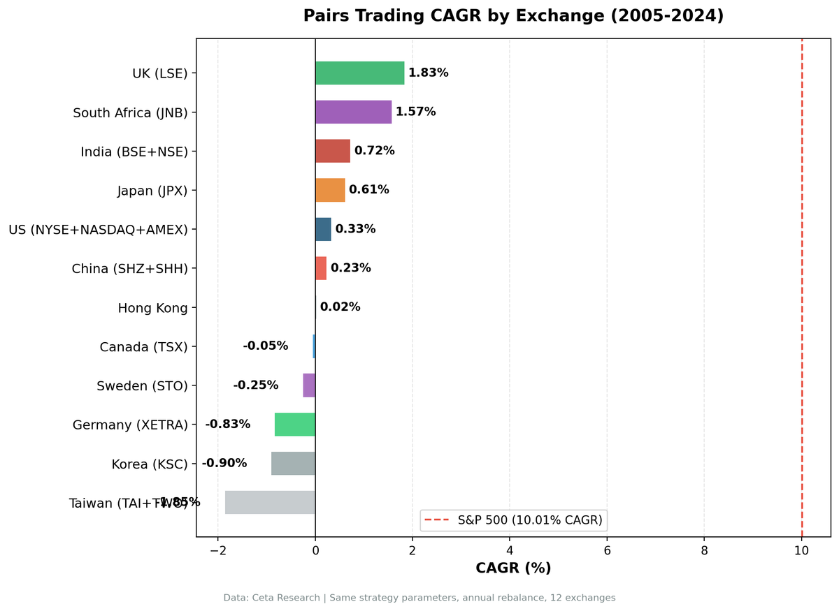
We ran the same pairs trading strategy on 11 exchanges and tested it over 20 years (2005-2024). Every single exchange underperformed its local benchmark. That was expected. What wasn't expected was how different the results are across markets, and what those differences reveal about market structure.
Contents
- Method
- Full Results
- What Explains the Differences
- Cash rate is not the driver
- Japan: persistent correlation, unreliable reversion
- South Africa: high volatility, rough ride
- Taiwan: concentrated tech, permanent divergence
- Korea: similar problem, worse Sharpe
- Crisis Performance Across Markets
- Exchanges Excluded
- Current Pairs Screens
- Limitations
The best result was UK at +1.85% CAGR. The worst was Taiwan at -2.03%.
Method
The strategy follows the Gatev et al. (2006) framework with same-sector constraints. Each year, we identify pairs within the same sector where the trailing correlation is 0.70 or higher. We use an OLS hedge ratio, enter when the z-score crosses +/-1.5, and exit at mean reversion or year-end. Returns are equal-dollar market-neutral: one long, one short, per pair. Next-day close execution (MOC).
Annual reconstitution. No leverage. Each exchange is benchmarked against its local index (Nikkei for Japan, FTSE for UK, etc.). SPY serves as a secondary cross-market reference.
The same code ran on all 11 exchanges. No universe-specific tuning.
Full Results
| Exchange | CAGR | Sharpe | Max Drawdown | Cash Years | Avg Pairs | Local Benchmark |
|---|---|---|---|---|---|---|
| LSE (UK) | +1.85% | -0.200 | -10.39% | 13/20 (65%) | 4.6 | FTSE 100 |
| JPX (Japan) | +0.61% | +0.131 | -11.18% | 1/20 (5%) | 6.3 | Nikkei 225 |
| TSX (Canada) | +0.19% | -0.600 | -8.64% | 5/20 (25%) | 5.7 | TSX Composite |
| HKSE (Hong Kong) | +0.09% | -0.749 | -13.92% | 8/20 (40%) | 5.7 | Hang Seng |
| SHZ+SHH (China) | -0.25% | -0.867 | -13.70% | 8/20 (40%) | 6.5 | SSE Composite |
| STO (Sweden) | -0.25% | -0.393 | -16.72% | 8/20 (40%) | 5.2 | SPY* |
| NYSE+NASDAQ+AMEX (US) | -0.50% | -0.813 | -18.39% | 6/20 (30%) | 5.4 | S&P 500 |
| JNB (South Africa) | -0.47% | -0.782 | -46.91% | 5/20 (25%) | 6.8 | SPY* |
| XETRA (Germany) | -0.83% | -1.184 | -16.14% | 14/20 (70%) | 4.8 | DAX |
| KSC (Korea) | -0.90% | -0.976 | -20.83% | 9/20 (45%) | 4.8 | KOSPI |
| TAI+TWO (Taiwan) | -2.03% | -0.417 | -35.31% | 13/20 (65%) | 4.9 | TAIEX |
JPX Sharpe computed using Japan's 0.1% risk-free rate. At a uniform 2% RFR, Japan's Sharpe falls to approximately -0.35.
China results are theoretical. See "Exchanges Excluded" section for the India and China short-selling caveats.
*Sweden and South Africa lack local index price data in FMP. SPY used as fallback benchmark.
What Explains the Differences
Cash rate is not the driver
The UK has 65% cash years and the best CAGR. Germany has 70% cash years and one of the worst CAGRs. If "pairs not firing" were uniformly bad, both should look similar.
They don't. When UK pairs do fire, they work. UK has a long-established institutional arbitrage culture, and sector divergences within the LSE tend to be transient. Germany's pairs fire less often, and when they do fire, the reversion is weaker. The German market's concentration in a few large-cap industrials and chemicals creates pairs that can diverge on fundamental grounds, not just noise.
Japan: persistent correlation, unreliable reversion
Japan sits at 5% cash (most active market in the set) with 0.61% CAGR. The keiretsu cross-holding structure creates stocks that move together for structural reasons. That gives you high correlation. It doesn't give you mean reversion. When a keiretsu pair diverges, it can stay diverged because the divergence reflects a real shift in the group's priorities, not a temporary pricing error.
The +0.131 Sharpe in Japan looks deceptively close to positive, but that's entirely a function of the near-zero risk-free rate. At a 2% RFR, Japan is just as negative as the others.
South Africa: high volatility, rough ride
South Africa's -0.47% CAGR with a -46.91% max drawdown tells a difficult story. In 2011, the rand fell 16% against the dollar, and sector divergences created paired positions that moved adversely. These weren't pricing errors correcting, they were fundamental events unfolding across correlated pairs simultaneously. The -30.32% loss in 2011 was the single worst year of any exchange in this backtest.
Taiwan: concentrated tech, permanent divergence
Taiwan at -2.03% with -35.31% max drawdown is the worst result. The exchange is dominated by the semiconductor supply chain. Companies that look highly correlated in calm periods (TSMC vs. peers, memory vs. logic) can diverge sharply and permanently when global tech cycles shift. The 2022 downcycle, the AI infrastructure buildout, US-China supply chain restructuring, all of these hit Taiwan's tech-heavy sectors asymmetrically. Annual-hold pairs don't close when the divergence is structural.
Korea: similar problem, worse Sharpe
Korea at -0.90% and -0.976 Sharpe mirrors the Taiwan dynamic. Heavy concentration in electronics and chemicals, with frequent structural breaks. The chaebol structure also means correlated pairs are correlated for ownership reasons, not business reasons. When one leg gets a conglomerate-level shock, the pair doesn't revert.
Crisis Performance Across Markets
2008 was the standout year for pairs trading everywhere. The market-neutral structure held. When both legs are shorted and longed within the same sector, broad market declines affect both positions. Most exchanges posted positive or flat returns that year while local benchmarks fell 30-40%.
This is the academic case for market-neutral pairs: it doesn't promise alpha, but it does provide crisis insulation. Across all 11 exchanges, 2008 was the year the strategy looked most useful.
The problem is consistency. After 2008, returns across exchanges fragmented. The 2010s were a sustained equity bull market, and the opportunity cost of holding a cash-heavy market-neutral strategy versus riding the beta was significant. Most exchanges saw cash rates climb as correlation screens tightened during low-volatility trending regimes.
The Do and Faff (2010) finding holds: algorithmic trading compressed pairs arbitrage opportunities substantially after 2002. Our 2005-2024 window captures only the compressed era, and the returns reflect it.
Exchanges Excluded
SIX (Switzerland) is excluded from this comparison. In 2007, the Swiss exchange produced a +56.72% single-year return from 5 pairs, which appears M&A-related. Under the annual-hold model, a pair involving an acquisition target will show abnormal returns when the deal closes. We didn't include SIX because that single year distorts the full-period CAGR in a way that isn't attributable to the strategy signal.
SET (Thailand) and SES (Singapore) both show 18 of 20 cash years. With the correlation and same-sector constraints, neither market produces enough qualifying pairs to run meaningfully. Reporting a 2-year sample would be misleading.
BSE+NSE (India) shows 15 of 20 cash years and is excluded from this comparison. More importantly, India has significant short-selling restrictions on equity. The short leg of a pairs trade often can't be executed at market prices. Results are theoretical even in active years. We ran the backtest for completeness, but the strategy isn't actionable in India as structured.
China (SHZ+SHH) is included in the table above, but the same short-selling caveat applies. A-share short selling was heavily restricted for domestic accounts throughout most of the 2005-2024 period, and international access was limited. The -0.25% CAGR is theoretical. It's shown because the methodology ran cleanly and the comparison is interesting, not because it's replicable.
Current Pairs Screens
The query below identifies current same-sector pairs with trailing correlation above 0.70 using FMP warehouse data. You can run it directly in the Ceta Research data explorer.
WITH price_data AS (
  SELECT
    p.exchange,
    p.sector,
    s.symbol,
    s.date,
    s.adjClose
  FROM stock_eod s
  JOIN profile p ON s.symbol = p.symbol
  WHERE s.date >= CURRENT_DATE - INTERVAL '365 days'
    AND p.exchange IN ('NYSE', 'NASDAQ', 'AMEX')
    AND p.sector IS NOT NULL
    AND s.adjClose > 0
),
returns AS (
  SELECT
    exchange,
    sector,
    symbol,
    date,
    adjClose / LAG(adjClose) OVER (PARTITION BY symbol ORDER BY date) - 1 AS daily_return
  FROM price_data
),
pair_corr AS (
  SELECT
    a.exchange,
    a.sector,
    a.symbol AS symbol_a,
    b.symbol AS symbol_b,
    CORR(a.daily_return, b.daily_return) AS correlation,
    COUNT(*) AS obs
  FROM returns a
  JOIN returns b
    ON a.date = b.date
    AND a.sector = b.sector
    AND a.symbol < b.symbol
  WHERE a.daily_return IS NOT NULL
    AND b.daily_return IS NOT NULL
  GROUP BY a.exchange, a.sector, a.symbol, b.symbol
  HAVING COUNT(*) >= 200
)
SELECT
  exchange,
  sector,
  symbol_a,
  symbol_b,
  ROUND(correlation::NUMERIC, 3) AS correlation,
  obs AS trading_days
FROM pair_corr
WHERE correlation >= 0.70
ORDER BY correlation DESC
LIMIT 100;
Shareable link: cetaresearch.com/data-explorer?q=FHNWEr6zkK
Limitations
Annual reconstitution is the biggest simplification. Real pairs traders reconstitute more frequently, especially after structural breaks. The annual model holds pairs that have stopped working.
No transaction costs on most non-US exchanges. Bid-ask spread and borrow cost on the short leg would reduce returns further, particularly in less liquid markets (JNB, Taiwan, Korea).
Look-ahead bias in pair selection is controlled by using trailing data only, but the same-sector constraint assumes sector classifications are stable. They're not. Reclassifications mid-year create retrospective pairs that wouldn't have been identified at the time.
Short-selling restrictions affect China, India, and historically Korea and Taiwan. Strategies that require a short leg can't be assumed executable at model prices in these markets.
Local benchmarks vs SPY. Each exchange is now benchmarked against its own local index. This is methodologically correct (same currency, same market risk) but makes cross-exchange comparisons less direct. The table uses local benchmarks for individual exchange analysis. When comparing across exchanges, note that the Sharpe ratios use different risk-free rates.
Data: FMP warehouse, 2005-2024. Next-day close execution (MOC). Each exchange benchmarked against its local index.